![]()
Stormwater modeling, models and calculators, and calculating credits-combined
The foundation of stormwater management is an understanding of how a particular land area and drainage system can affect or be affected by the stormwater passing through it. In particular, when alterations to the land area or drainage network are planned or being made, stormwater managers need to understand and anticipate how the alteration is likely to affect the volume, flow rate, and quality of runoff moving through the system, and in turn, how the stormwater is likely to impact the people, property, and natural resources of the area. Modeling is a tool that can be used to understand and evaluate these complex processes involving stormwater runoff.
Contents
- 1 Purpose of stormwater modeling
- 2 Types of models
- 3 Limitations of modeling and the importance of calibration
- 4 Minnesota model input guide
- 4.1 Model input guidance
- 4.1.1 Precipitation
- 4.1.2 Rainfall distribution
- 4.1.3 Runoff estimation
- 4.1.4 Event Mean Concentrations
- 4.1.5 Climate trends
- 4.2 Resources for model input data
- 4.3 Sources of Data
- 4.1 Model input guidance
- 5 References
- 6 Defining Model Objectives and Selecting a Stormwater Model
- 7 Summary of Common Stormwater Models
- 7.1 Rational method
- 7.2 HEC-HMS
- 7.3 TR-20
- 7.4 Win TR-55
- 7.5 HEC-RAS
- 7.6 WSPRO
- 7.7 CULVERTMASTER
- 7.8 FLOWMASTER
- 7.9 HydroCAD
- 7.10 PondPack
- 7.11 SWMM-Based programs (SWMM5, PC-SWMM, InfoSWMM, MikeUrban)
- 7.12 XPSWMM
- 7.13 WinSLAMM
- 7.14 P8
- 7.15 BASINS
- 7.16 PONDNET
- 7.17 WiLMS
- 7.18 Bathtub
- 7.19 WASP
- 7.20 SUSTAIN
- 7.21 MIDS Calculator
- 7.22 STEPL
- 7.23 Virginia runoff reduction method
- 7.24 USEPA National Stormwater Calculator
- 7.25 Autodesk Civil 3D
- 8 Table summarizing models by model type
- 9 Table summarizing information for different models
- 10 Definition of credit
- 11 Applicability of credits
- 12 Consistency in calculating credits
- 13 Concerns/disadvantages of crediting
- 14 Is my community ready for credits?
- 15 Adapting credits for local use
- 16 Integrating credits into the local development review process
- 17 What is the pre-development condition?
Purpose of stormwater modeling
Some kind of stormwater model is needed whenever an estimate of the expected volume, rate, or quality of stormwater is desired. Modeling is also often necessary for the proper design of stormwater Best Management Practices (BMPs) and hydraulic structures and for evaluation of the effectiveness of water quality treatment by BMPs. If monitoring data exists for the specific combination of precipitation and site conditions under consideration, modeling may not be necessary. However, in many cases the conditions to be analyzed do not fit precisely with monitoring conditions and modeling will be necessary.
In general, models can be physical or numerical. A physical model is a constructed replica of the system, whereas a numerical model is based on equations that approximate the processes occurring in the system. Typically, it is not realistic to construct a physical model that would provide reliable hydrologic predictions for a watershed or drainage system, so numerical (nearly always computer-based) models are the standard tool for stormwater management.
Note that this Manual cannot possibly contain a thorough analysis of modeling. Instead, the purpose is to introduce a stormwater manager to the terms of modeling and some cursory assessment of model calibration. For a brief description of various available models, see Available stormwater models and selecting a model.
In practice, stormwater models are most commonly used either as planning and decision-making aids for water management authorities, or as tools for developers who wish to design for and demonstrate compliance with regulations governing protection of water and waterways. They are used, for example, to predict
- water quality effects of various land management scenarios;
- effects of water control structures on water surface elevations in a channel;
- performance of stormwater management structures such as ponds, wetlands, and trenches;
- wetland impacts resulting from channel excavation; and
- lateral extents of a floodplain along a channel.
These examples show some of the potential uses of modeling, but the list is by no means exhaustive. Modeling in general is a versatile tool that can be applied to a large number of situations.
Types of models
The most commonly used stormwater models can generally be classified as either hydrologic, hydraulic, or water quality models.
- Hydrologic models are used to estimate runoff volumes, peak flows, and the temporal distribution of runoff at a particular location resulting from a given precipitation record or event. Essentially, hydrologic models are used to predict how the site topography, soil characteristics, and land cover will cause runoff either to flow relatively unhindered through the system to a point of interest, or to be delayed or retained somewhere upstream. Many hydrologic models also include relatively simple procedures to route runoff hydrographs through storage areas or channels, and to combine hydrographs from multiple watersheds.
- Hydraulic models are used to predict the water surface elevations, energy grade lines, flow rates, velocities, and other flow characteristics throughout a drainage network that result from a given runoff hydrograph or steady flow input. Generally, the output (runoff) from a hydrologic model is used in one way or another as the input to a hydraulic model. The hydraulic model then uses various computational routines to route the runoff through the drainage network, which may include channels, pipes, control structures, and storage areas. Combined hydraulic and hydrologic models provide the functions of both hydraulic models and hydrologic models in one framework. A combined model takes the results from the hydrologic portion of the model and routes it through the hydraulic portion of the model to provide the desired estimates.
- Water quality models are used to evaluate the effectiveness of a BMP, simulate water quality conditions in a lake, stream, or wetland, and to estimate the loadings to water bodies. Often the goal is to evaluate how some external factor (such as a change in land use or land cover, the use of best management practices, or a change in lake internal loading) will affect water quality. Parameters that are frequently modeled include total phosphorus, total suspended solids, and dissolved oxygen.
Limitations of modeling and the importance of calibration
Hydrologic, hydraulic, and water quality models are not exact simulations of the processes occurring in nature. Rather, they are approximate representations of natural processes based on a set of equations simplifying the system and making use of estimated or measured data. The accuracy of a model, therefore, is limited by the quality of the simplifications made to approximate the system processes and the quality of the input data. In some cases, the impact of these limitations can be reduced by using a more complex model or paying to acquire more or better input data. However, it is also important to recognize that oftentimes, it is simply not possible to significantly increase accuracy with such means, because the necessary computational and data collection technology does not exist, and in any case the climatic forces driving the simulation can only be roughly predicted. There also could be time and funding constraints.

Recognizing the high degree of error or uncertainty inherent in many aspects of stormwater modeling can help to focus efforts where they do the most good. Generally, the goal of stormwater modeling is to provide a reasonable prediction of the way a system will respond to a given set of conditions. The modeling goal may be to precisely predict this response or to compare the relative difference in response between a number of scenarios. The best way to verify that a model fulfills this need (to the required degree of accuracy) is to check it against actual monitoring data or observations.
The process of model calibration involves changing the estimated input variables so that the output variables match well with observed results under similar conditions. The process of checking the model against actual data can vary greatly in complexity, depending on the confidence needed and the amount of data available. In some cases, the only feasible or necessary action may be a simple “reality check,” using one or two data points to verify that the model is at least providing results that fall within the proper range. In other cases, it may be necessary to perform a detailed model calibration, to ensure the highest possible accuracy for the output data. For some models, calibration is unnecessary due to the design of the model.
Calibration should not result in the use of model parameters that are outside a reasonable range. Additionally, models should not be calibrated to fit so tightly with observed data that the model loses its flexibility to make estimates under other climatic conditions.
Minnesota model input guide
The section on unified sizing criteria outlines recommendations for sizing best management practices. The following sources of information will allow designers to use the above referenced models for estimating hydrologic, hydraulic, or water quality parameters.
Model input guidance
Models range from simple to complex. Modelers should refer to the page discussing available models for an up-to-date listing of models most frequently used in Minnesota. The following discussion provides a brief background on model input data and indicates where to find model input data. Simple models may require some of the following data be input, while complex models may require additional input that is not described in this section. Designers and modelers are encouraged to review the sources of the information presented for more detailed information.
Precipitation
Models are often required to predict the effects of a wide range of precipitation events, ranging from water quality events (equal to a precipitation depth of approximately 1 inch) to an extreme event such as back-to-back 100 year rainfalls. The purpose of this section is to describe the information that modelers will need to predict the rainfall and runoff for these events which, in turn, may be used to size a BMP, predict downstream effects, or some other hydraulic purpose. These events are further defined in the Unified Sizing Criteria section of the Minnesota Stormwater Manual.
Stormwater models are used for the fundamental purpose of evaluating existing stormwater facilities for both hydraulic performance and water quality performance, and sizing alternative facilities to meet level of service objectives. Historically stormwater designs were intended to convey the runoff from a major event, typically the 1 percent storm, casually termed the 100-year event. Design engineers typically make use of precipitation exceedance probabilities to calculate the risks associated with lack of storm sewer capacity, channel erosion, over-bank flooding, and extreme flooding. A storm magnitude with a return period (T) has the probability of being equaled or exceeded in any given year equal to 1/T. For example a “100-year” event at a given location has a 1/100 (or 1 percent) chance of being equaled or exceeded in any given year.
More recently, since the mid-1990’s, stormwater facilities must also be sized to manage the runoff from small storms, generally with precipitation volumes less than a 1-year event, for the purpose of treating the runoff to meet water quality objectives. Stormwater treatment and streambank erosion control require effective management of a long-term sequence of rainfall runoff events rather than performance under a single design storm event.
All stormwater models require the input of hydrologic parameters, typically in the form of rainfall; parameters to convert rainfall to runoff such as land use and infiltration; and relationships that yield equivalent rainfall-runoff volumes, intensities, durations and frequencies. The modeling approach will vary based on whether the model is set up to predict the runoff of a single event or a series of events, or a long-term continuous simulation. Single events are important for the sizing of a conveyance system and a BMP. Continuous simulation models are important when assessing the downstream effects of a stormwater discharge. For example channel erosion protection needs to be based more on continuous simulations of more frequent storms to properly represent the duration of erosive periods, particularly if detention used to control peak rate of runoff with limited volume control (WEF, 2012).
This section lays out the types of statistical precipitation data that is available.
Historic and current statistical precipitation studies
Statistical evaluations of precipitation volume, intensity, duration, and frequency have been performed over the past 50 years, with the more recent evaluations benefiting from a larger, more statistically accurate database of measured precipitation data.
Until recently, the most commonly referenced precipitation frequency study in Minnesota was Technical Paper No. 40 (TP-40). The precipitation-frequency estimates in NOAA Atlas 14 supersede the estimates produced in TP-40, as well as those in TP-49 and NWS HYDRO-35. These historic studies are included for purpose of comparison and transition to Atlas 14, as required by the Minnesota Department of Transportation and an increasing number of watershed districts/watershed management organizations. Studies associated with approximating the precipitation statistics for areas within Minnesota are included below, along with their publication dates and links to their documentation.
- National Oceanic and Atmospheric Administration (NOAA) Atlas 14: Precipitation-Frequency Atlas of the United States, Volume 8 (2013)
- Minnesota Department of Transportation (MnDOT), Intensity of Extreme Rainfall Events over Minnesota (1998)
- Metropolitan Council’s Precipitation Frequency Analysis for the Twin Cities Metropolitan Area (1995)
- Midwest Climate Center and Illinois State Water Survey (ISWS) Bulletin 71: Rainfall Frequency Atlas of the Midwest (1992)
- NOAA Technical Memorandum NWS HYDRO-35: Five- to 60-Minute Precipitation Frequency for the Eastern and Central United States (1977)
- Weather Bureau Technical Paper No. 49: Two- to Ten-Day Precipitation for Return Periods of 2 to 100 Years in the Contiguous United States (1964)
- Weather Bureau Technical Paper No. 40: Rainfall Frequency Atlas of the United States for Durations from 30 Minutes to 24 Hours and Return Periods from 1 to 100 Years (1961)
In addition to these frequency analysis studies, an impressive source of historical (and current) precipitation data and other climate data for Minnesota has been compiled by the Minnesota Climatology Working Group.
Prior to development of Atlas 14 in 2013 the more recent work listed above was developed to test and/or validate the TP-40 findings include precipitation frequency studies conducted by the Midwest Climate Center (Huff and Angels’ 1992 Bulletin 71), Metropolitan Council’s Precipitation Frequency Analysis for the Twin Cities Metropolitan Area (study updates in 1984, 1989, and 1995), and Mn/DOT’s November 1998 study Intensity of Extreme Rainfall over Minnesota in coordination with Richard Skaggs from the University of Minnesota. The major differences between the NOAA Atlas 14 analysis and those performed in previous studies include the following.
- NOAA Atlas 14 uses an increased number of precipitation stations in the statistical analysis
- For Minnesota, 285 stations were used in NOAA Atlas 14 that had daily precipitation recorded, compared to 110 such stations used in the TP-40 study
- For Minnesota, 87 stations were used in NOAA Atlas 14 that had precipitation recorded on an interval smaller than a day, compared to 33 such stations used in the TP-40 study
- NOAA Atlas 14 includes additional precipitation records
- NOAA Atlas 14 includes precipitation data through 2012-2013
- TP-40 was published in 1960, TP-49 in 1964, NWS HYDRO-35 in 1977 and ISWS Bulletin 71 in 1992; this equates to at least 21 to 53 additional years of data in Atlas 14
- NOAA Atlas 14 uses a more robust statistical analysis
- Multiple distribution functions were analyzed for each region; most appropriate function was used in the final analysis
- Statistical analysis took into account precipitation from nearby stations and topography
NOAA Atlas 14
In April 2013, the National Oceanographic and Atmospheric Administration (NOAA) released Atlas 14: Precipitation-Frequency Atlas of the United States, Volume 8, Version 2.0. The precipitation frequency estimates contained in Volume 8 were developed for eleven Midwestern states, including Minnesota. As part of this new analysis, precipitation depths for ten separate recurrence intervals and 19 separate storm durations were produced. The recurrence intervals and storm durations are noted below.
NOAA Atlas 14 recurrence intervals and storm durations
Link to this table.
| Recurrence intervals | Storm durations |
|---|---|
| 1-year | 5-minute |
| 2-year | 10-minute |
| 5-year | 15-minute |
| 10-year | 30-minute |
| 25-year | 60-minute |
| 50-year | 2-hr |
| 100-year | 3-hr |
| 200-year | 6-hr |
| 500-year | 12-hr |
| 1000-year | 24-hr |
| 2-day | |
| 3-day | |
| 4-day | |
| 7-day | |
| 10-day | |
| 20-day | |
| 30-day | |
| 45-day | |
| 60-day |
The results of the revised precipitation-frequency analysis can be found on NOAA’s Precipitation Frequency Data Server (PFDS). The site is intuitive, allowing the user to select any location within the State of Minnesota and obtain precipitation depths for the duration and frequency combinations noted in the table above. The site also provides several supplementary documents for the specific area that the user may find useful, including isopluvial maps, temporal distributions, and a seasonality analysis. MnDOT has produced several documents and presentations regarding the use of NOAA Atlas 14 and the PFDS that can be found on their website, including Technical Memorandum 15-10-B-02, which summarizes the shift to use of Atlas 14.

Snowfall was considered in the NOAA Atlas 14 analysis, both in the form of snow or when converted to snow water. However, it was determined that the difference in the final precipitation frequency estimates between snow forms was trivial for all stations across Minnesota for all durations. Also, although noted that a regional approach was completed during the statistical analysis by using precipitation values from nearby stations, the results on the PFDS are point estimates. In order to apply these precipitation estimates over an area (i.e., a watershed), appropriate areal reduction factors must be used. These reduction factors are typically a function of the size of area and the duration of the precipitation.
In general, the results of NOAA Atlas 14 show increased precipitation depths when compared to results published in TP-40, especially at higher recurrence intervals. Much of southern Minnesota show a precipitation estimate increase as much as 2 inches for the 100-year 24-hour event.
To show a comparison between the precipitation estimates from NOAA Atlas 14, TP-40, and Bulletin 71, six sites across Minnesota were selected.
- Minneapolis-St. Paul International Airport
- Rochester airport
- St. Cloud Airport
- Lamberton
- Cloquet
- Itasca County
The table below shows precipitation estimates (in inches) for the 24-hour duration from the three publications. Three recurrence intervals were selected, signifying the events that may be of interest for engineers when examining the risk associated with channel erosion (2-year event), storm sewer surcharging (10-year event), or flood hazard areas (100-year event). The table shows that precipitation estimates in NOAA Atlas 14 represent a 0 to 9 percent increase as compared to the other two studies for the 2-year event, a 0 to 15 percent increase for the 10-year event, and a 7 to 37 percent increase for the 100-year event.
Comparison of precipitation totals from TP-40, Bulletin 71, and Atlas 14. All values are in inches per hour.
Link to this table
| Recurrence interval | Method | Cloquet | Itasca county | Lamberton | Minneapolis-St. Paul Airport | Rochester Airport | St. Cloud Airport |
|---|---|---|---|---|---|---|---|
| 2-year | TP-40 | 2.5 | 2.4 | 2.8 | 2.8 | 2.9 | 2.6 |
| Bulletin 71 | 2.65 | 2.41 | 2.69 | 2.65 | 2.84 | 2.54 | |
| Atlas 14 | 2.69 | 2.61 | 2.72 | 2.83 | 2.93 | 2.68 | |
| 10-year | TP-40 | 3.8 | 3.7 | 4.2 | 4.2 | 4.3 | 4.1 |
| Bulletin 71 | 3.69 | 3.58 | 3.81 | 3.69 | 4.08 | 3.68 | |
| Atlas 14 | 3.87 | 3.90 | 4.03 | 4.23 | 4.46 | 3.92 | |
| 100-year | TP-40 | 5.3 | 5.3 | 6.0 | 6.0 | 6.1 | 5.8 |
| Bulletin 71 | 5.46 | 5.88 | 5.94 | 5.46 | 5.76 | 5.72 | |
| Atlas 14 | 6.22 | 6.30 | 6.75 | 7.49 | 7.85 | 6.34 |
While NOAA Atlas 14 is considered a robust study that utilizes the most recent precipitation data, its use may not be required at this time. MnDOT is requiring the use of Atlas 14 for trunk highway projects, where feasible. Many watershed organizations throughout the state are in the process of reviewing the data in Atlas 14 and are considering whether to incorporate this new precipitation data into their requirements. Modelers are encouraged to contact the appropriate organization (e.g., MPCA, MNDOT, watershed organizations) for information on the usage of Atlas 14. The links below show the location of watershed organizations throughout the state and provide a link to their individual websites.
- BWSR Local Government Units: Watershed District
- BWSR Local Government Units: Watershed Management Organization
Extreme flood events
Because a spring melt event generates a large volume of water over an extended period of time, evaluation of the snowmelt event for channel protection and over-bank flood protection is generally not as important as the extreme event analysis. This warrants attention because of the possibility that a major melt flooding event could, and sometimes does, happen somewhere in the state.
Conservative design for extreme storms can be driven by either a peak rate or volume event depending upon multiple hydraulic factors. Therefore, depending upon the situation, either the 100-yr, 24-hr rain event or the 100-yr, 10-day snowmelt runoff event can result in more extreme conditions. For this reason, both events should be analyzed.
Protocol for simulation of the 100-yr, 24-hr rainfall event is well established in Minnesota. High water elevations (HWL) and peak discharge rates are computed with storm magnitudes based on TP-40 frequency analysis and the SCS Type II storm distribution.
Protocol has been established for the analysis of HWL and peak discharge resulting from a 7.2 inch 100-yr, 10-day snowmelt runoff event. However, this event has received a considerable amount of criticism. Although not well documented, it is thought that the theoretical snowmelt event was devised by assuming a 6 inch 100-yr, 24-hr rainfall event occurs during a 10-day melt period in which 1 foot of snow (with a 10 percent moisture content) exists at the onset. A typical assumption accompanying the event is that of completely frozen ground (no infiltration) during the melt period for which the result is 100 percent delivery of volumes. So what do we use? Climate records show that the highest rain event during this common melt period over the past 100+ years was 4.75 inches. An alternative method to consider is to add 4.75 inches of precipitation to the site’s snowmelt volume (including infiltration). Designers should compare this to the 7.2 inch, 10-day snowmelt volumes and then determine which is best for the site.
Protocols for computation of extreme snowmelt events should be established as part of a state-wide precipitation study that has been discussed to update TP-40.
Water quality event
Most models developed will need to assess the pollutant removal and volume management of a BMP. Small storms are the focus of these water quality requirements because research has shown that pollution migration associated with frequently occurring events accounts for a large percentage of the annual pollutant load. The Minnesota Construction General Permit (CGP) as well as certain local regulatory agencies will require that developments retain the runoff generated from a rainfall up to 1 inch in depth.
Rain events between 0.5 inches and 1.5 inches are responsible for about 75 percent of runoff pollutant discharges (MPCA, 2000). The rainfall depth corresponding to 90 percent and 95 percent of the annual total rainfall depth shows surprising consistency among six stations chosen to represent regional precipitation across the State. The six stations analyzed were Minneapolis/St. Paul International Airport, St. Cloud Airport, Rochester Airport, Cloquet, Itasca County, and the Lamberton SW Experiment Station. The rainfall depth which represents 90 percent and 95 percent of runoff producing events was 1.09 inches (+/- 0.04 inches) and 1.46 inches (+/- 0.08 inches), respectively. This rainfall depth can be used for water quality analysis throughout the state (EOR, 2005).
The potential exists that a snowmelt event may need to be modeled for the purpose of assessing the pollutant removal by a BMP or for the pollutant loading from a large watershed containing multiple BMPs. The following technique may be utilized to analyze snowmelt.
Technical Bulletin 333, Climate of Minnesota (Kuehnast, 1982), shows that the average annual date of snowmelt can be represented by the last date of a 3 inch snow cover. This document also includes figures that allow estimation of the average depth of snowpack at the start of spring snowmelt plus the water content of the snowpack during the month of March.
The estimated infiltration volume can be determined from research in cold climates by Baker (Lyons-Johnson, 1997), Buttle and Xu (1988), Bengtsson (1981), Dunne and Black (1971), Granger et al. (1984) and Novotny (1988). This research shows that infiltration does in fact occur during a melt at volumes that vary considerably depending upon multiple factors including: moisture content of the snow pack, soil moisture content at the time the soil froze, plowing, sublimation, vegetative cover, soil properties, and other snowpack features. For example, snowmelt investigations by Granger et al. (1984) took measurements from 90 sites, located in Saskatchewan Canada, representing a wide range of land use, soil textures, and climatic conditions. From this work, general findings showed that even under conservative conditions (wet soils, ~35 percent moisture content, at the time of freeze) about 0.4 inches of water infiltrated during the melt period from a one-foot snowpack with a 10 percent moisture content (1.2 inches of equivalent moisture) in areas with pervious cover. This would not apply to impervious surfaces (see Overview of basic stormwater concepts). Other procedures for estimating water quality treatment volume based on annual snow depth are described by the Center for Watershed Protection (CWP) (Caraco and Claytor, 1997).
For purposes of determining the volume of runoff or snowmelt that should be managed by the site BMPs, designers must make two water quality volume computations: snowmelt and rainfall runoff. The BMP would then be sized for the larger of the two results. Areas with low snowfall will likely find that the rainfall based computations are the larger value, while those areas with greater snowpack will find that snowmelt is larger. In some cases snowmelt would be selected as the design parameter for computing the volume, whereas other options lead to rainfall as the critical design parameter (see Unified sizing criteria).
Between 2011 and 2013, new performance goals were developed as part of the Minimal Impact Design Standards (MIDS). The precipitation depth is applied over all new and/or fully reconstructed impervious areas to determine the volume that must be retained on site for water quality purposes. The MIDS performance standards apply to sites creating 1 or more acres of impervious surface.
- New development (nonlinear): 1.1 inches from all new impervious surfaces
- Redevelopment (nonlinear): 1.1 inches from all new and/or fully reconstructed impervious surfaces
- New development/redevelopment, linear: larger of
- 0.55 inches from all new and/or fully reconstructed impervious surfaces
- 1.1 inches from the net increase in impervious area
Rainfall distribution
Storm distribution is a measure of how the intensity of rainfall varies over a given period of time. For example, in a given 24 hour period, a certain amount of rainfall is measured. Rainfall distribution describes how that rain fell over that 24 hour period; that is, whether the precipitation occurred over a one hour period or over the entire 24 hours. A plot of the distribution of the rainfall will determine the timing and extent of the peak rainfall, which is assumed to represent the timing of the peak runoff generated by the rainfall. This information is developed for models that predict the peak flow for the purpose of sizing the conveyance capacity of a storm sewer or a BMP.
Historic rainfall records are not considered reliable for the purpose of developing rainfall distribution curves (called hyetographs) over a wide range of watershed sizes that are typically evaluated in a single computer simulation. The most reliable approach to predict the resulting runoff from a rain event would be to assess the streamflow data against the rainfall to understand runoff. It is rare that streamflow records are available. Therefore hydrologists have developed approaches that are used to develop “synthetic” rainfall distributions to equate rainfall statistics to runoff statistics.
The advantage of using a synthetic event is that it is appropriate for determining both peak runoff rate and runoff volume. The most commonly used approaches are described in this section. A MnDOT memorandum recommends use of a rainfall distribution derived from Atlas 14 data or the NRCS MSE 3 distribution, both of which are described below.
Type II rainfall distribution

The standard rainfall distribution used in Minnesota was the SCS (now the NRCS) Type II distribution. This distribution was developed in the 1960s using the precipitation-frequency estimates contained in Technical Paper No. 40 (described in Precipitation). The release of NOAA Atlas 14 provides updated and more reliable precipitation-frequency estimates. The Type II rainfall distribution was created using data over a large geographic area; therefore, the resulting peak discharge for a smaller area may be over- or under-estimated. Consequently, the use of the SCS Type II rainfall distribution is becoming archaic. The Minnesota Department of Transportation (MnDOT) is recommending the use of NOAA 14 data to create a nested rainfall distribution, as described below. Other distributions are available; the Huff Distribution (as described in Bulletin 71) and updated distributions from NRCS are described further in this section.
Nested distribution using NOAA Atlas 14 precipitation-frequency data
The precipitation-frequency data presented in NOAA Atlas 14 can be used directly to develop a rainfall distribution. The basis of the distribution is to nest the high-intensity, short duration precipitation values within the lower-intensity, longer duration values. For study basins with a time of concentration less than 24 hours, a 24-hour rainfall distribution is appropriate since the largest peak discharge is generally produced when the storm duration is equal to the time of concentration. A cumulative discharge curve for each desired frequency is produced by taking the fraction of each storm duration over the 24-hour duration and centering it around a 12-hour time period. The fractions of the NOAA Atlas 14 precipitation depths for each duration over the 24-hour duration are subsequently centered around the 50 percent ratio. Consult the MnDOT website for presentations and tutorials on how to create the nested rainfall distribution.
Bulletin 71 rainfall distribution
The Midwest Atlas, also called Bulletin 71, has not been widely used in Minnesota. The rainfall distribution information presented in this section is included for the purpose of comparison for those modelers utilizing Bulletin 71, or considering transitioning from Bulletin 71 to Atlas 14. The Bulletin 71 Rainfall distribution was developed by examining the time-distribution characteristics of storms in Illinois. According to Bulletin 71, the time-distribution relationships should be applicable to the other Midwestern states studied, including Minnesota. Four distribution curves were developed and classified as first-, second-, third-, and fourth-quartile storms based on which quarter of the total storm period the greatest percentage of the rainfall occurred. The area over which the rain fell was also examined. The following table shows the median time distributions for all four quartiles for both rainfall at a point, and rainfall over a 10- to 50-square mile area.
Cumulative percent storm rainfall Bulletin 71
Link to this table.
| Cumulative percent of storm time | Rainfall at a point | Rainfall on areas of 10 to 50 square miles (%) | ||||||
|---|---|---|---|---|---|---|---|---|
| 0 | 0 | 0 | 0 | 0 | 0 | 0 | 0 | 0 |
| 5 | 16 | 3 | 3 | 2 | 12 | 3 | 2 | 2 |
| 10 | 33 | 8 | 6 | 5 | 25 | 6 | 5 | 4 |
| 15 | 43 | 12 | 9 | 8 | 38 | 10 | 8 | 7 |
| 20 | 52 | 16 | 12 | 10 | 51 | 14 | 12 | 9 |
| 25 | 60 | 22 | 15 | 13 | 62 | 21 | 14 | 11 |
| 30 | 66 | 29 | 19 | 16 | 69 | 30 | 17 | 13 |
| 35 | 71 | 39 | 23 | 19 | 74 | 40 | 20 | 15 |
| 40 | 75 | 51 | 27 | 22 | 78 | 52 | 23 | 18 |
| 45 | 79 | 62 | 32 | 25 | 81 | 63 | 27 | 21 |
| 50 | 82 | 70 | 38 | 28 | 84 | 72 | 33 | 24 |
| 55 | 84 | 76 | 45 | 32 | 86 | 78 | 42 | 27 |
| 60 | 86 | 81 | 57 | 35 | 88 | 83 | 55 | 30 |
| 65 | 88 | 85 | 70 | 39 | 90 | 87 | 69 | 34 |
| 70 | 90 | 88 | 79 | 45 | 92 | 90 | 79 | 40 |
| 75 | 92 | 91 | 85 | 51 | 94 | 92 | 86 | 47 |
| 80 | 94 | 93 | 89 | 59 | 95 | 94 | 91 | 57 |
| 85 | 96 | 95 | 92 | 72 | 96 | 96 | 94 | 74 |
| 90 | 97 | 97 | 95 | 84 | 97 | 97 | 96 | 88 |
| 95 | 98 | 98 | 97 | 92 | 98 | 98 | 98 | 95 |
| 100 | 100 | 100 | 100 | 100 | 100 | 100 | 100 | 100 |
Modelers should assess which distribution is the best fit for the watershed being modeled. The Third Quartile distribution for the 24 hour event often is more appropriate for watersheds with longer times of concentration (10 to 50 square mile ones noted in Rainfall Frequency Atlas of the Midwest), while the First Quartile can be the better fit for a 6 hour distribution in a small urban watersheds of a few square miles or less.
A distribution similar study was completed in NOAA Atlas 14. The study noted that the majority of storms in the North Plains, which includes Minnesota, are first-quartile events, as shown in the following table. The NOAA Atlas 14 results presented on their Precipitation Frequency Data Server include temporal distributions for each of the quartile events for each area in Minnesota for the six-, 12-, 24-, and 96-hour durations.
Cumulative Percent of Storm Rainfall for Given Storm Type – Atlas 14. Source: U.S. Department of Commerce. NOAA Atlas 14, Precipitation-Frequency Atlas of the United States, Volume 8, Version 2, 2013.
Link to this table.
| Duration | All cases | First quartile cases | Second quartile cases | Third quartile cases | Fourth quartile cases |
|---|---|---|---|---|---|
| 6-hour | 8828 | 3967 (45%) | 2547 (29%) | 1554 (17%) | 760 (9%) |
| 12-hour | 9010 | 4593 (51%) | 2110 (23%) | 1505 (17%) | 802 (9%) |
| 24-hour | 8370 | 4170 (50%) | 1765 (21%) | 1378 (16%) | 1057 (13%) |
| 96-hour | 8415 (47%) | 3990 (47%) | 1551 (18%) | 1389 (17%) | 1485 (18%) |
NRCS Revised Rainfall Distributions
The NRCS has developed rainfall distribution curves for three NRCS distribution regions in Minnesota based on Atlas 14 data. These are available in spreadsheet format on the NRCS Minnesota website.
Rainfall Distribution Comparison
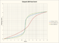
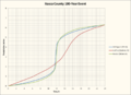
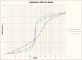
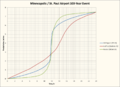
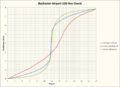
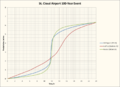
The figures below compare the SCS Type II, NOAA Atlas 14 Nested, and Huff (first quartile) cumulative rainfall distribution graphs for the 100-year event at the six locations that were assessed in 2005 for the first edition of the MN stormwater manual (EOR, 2005). Further information regarding rainfall distribution can be found on the NRCS Minnesota Hydrology and Hydraulics web page.
- Rainfall distribution comparison for 100-year, 24-hour precipitation event for 6 locations in Minnesota. Source: CDM Smith Click on an image for enlarged view.


Runoff estimation
As described in the Rainfall Distribution of this Minnesota Stormwater Manual, rainfall records are typically used to estimate the rate and volume of runoff that is generated for both large and small rain events. There are many factors that influence the generation of runoff as well as the prediction of runoff. The generation of runoff is influenced by soil type, moisture conditions of the soil, area of impervious cover, land slope, and other physical features. Models will utilize techniques to predict runoff which require the input of some or all of the parameters described in this section.
Runoff coefficient
The runoff coefficient is a unitless factor that represents the fraction of rainfall that becomes runoff. It is used in the Rational Method to estimate peak runoff rates for very small drainage areas, typically less than 50 acres (WEF, 2012). The simple equation for peak discharge (Q, in cubic feet per second) is Q=CiA, where C is a runoff coefficient, i is rainfall intensity in inches per hour, and A is drainage area in acres. The chosen value of C must represent losses to infiltration, detention, and antecedent moisture conditions. Additionally, C varies with the frequency of the rainfall event, with the smaller C values related to the smaller rain events. Tabled values for C are shown below for 5- to 10-year events.
Runoff coefficients for 5- to 10-year storms (Source: Haan et al., 1994)
Link to this table
| Land use description | Runoff coefficient (C) |
|---|---|
| Forest | |
| < 5% slope | 0.30 |
| 5 to 10% slope | 0.35 |
| > 10% slope | 0.50 |
| Open space | |
| < 2% slope | 0.05 to 0.10 |
| 2 to 7% slope | 0.10 to 0.15 |
| > 7% slope | 0.15 to 0.20 |
| Industrial | 0.50 to 0.90 |
| Residential | |
| Multi-family | 0.40 to 0.75 |
| Single family | 0.30 to 0.50 |
| Impervious areas | 0.70 to 0.95 |
| Row crops1 | |
| < 5% slope | 0.50 |
| 5 to 10% slope | 0.60 |
| > 10% slope | 0.72 |
| Pasture | |
| N 5% slope | 0.30 |
| 5 to 10% slope | 0.36 |
| > 10% slope | 0.42 |
1For clay and silt loam soils.
Curve numbers
Curve number (CN) is a unit-less parameter that represents the runoff potential of a specific land area for use in models that utilize the SCS method of predicting runoff. It was developed by the USDA Natural Resource Conservation Service (NRCS), formerly called the Soil Conservation Service (SCS). Although the name of the organization has changed, CN is still often referred to as “SCS Curve Numbers”. Curve numbers range from 0 to 100, with the smaller numbers representing low runoff potential and the higher numbers representing high runoff potential. The factors that are considered when selecting a CN include the following.
- Hydrologic Soil Group (HSG), which consist of four classifications (A, B, C, and D) grouped according to soil infiltration rates
- Cover type, such as pavement, grass, bare soil, etc.
- Treatment, a modification of cover type based on the management of the cover, such as contouring of agricultural lands, or mowing of urban parks.
- Hydrologic condition, representing the condition of cover type, including the density of plantings or degree of surface roughness
Additional information and CN tables are available from NRCS.
Curve number selection
Curve number tables are published in TR-55 (Urban Hydrology for Small Watersheds), but are also available in textbooks and within modeling software.
Curve numbers for antecedent moisture condition II (Source USDA-NRCS).
Link to this table
| A | B | C | D | |
|---|---|---|---|---|
| Meadow - good condition | 30 | 58 | 72 | 78 |
| Forest | ||||
| Poor | 45 | 66 | 77 | 83 |
| Fair | 36 | 60 | 73 | 79 |
| Good | 30 | 55 | 70 | 77 |
| Open space | ||||
| Poor | 68 | 79 | 86 | 89 |
| Fair | 49 | 69 | 79 | 84 |
| Good | 39 | 61 | 74 | 80 |
| Commercial 85% impervious | 89 | 92 | 94 | 95 |
| Industrial 72% impervious | 81 | 88 | 91 | 93 |
| Residential | ||||
| 1/8 acre lots (65% impervious) | 77 | 85 | 90 | 92 |
| 1/4 acre lots (38% impervious) | 61 | 75 | 83 | 87 |
| 1/2 acre lots (25% impervious) | 54 | 70 | 80 | 85 |
| 1 acre lots (20% impervious) | 51 | 68 | 79 | 84 |
| Impervious areas | 98 | 98 | 98 | 98 |
| Roads (including right of way) | ||||
| Paved | 83 | 89 | 92 | 93 |
| Gravel | 76 | 85 | 89 | 91 |
| Dirt | 72 | 82 | 87 | 89 |
| Row crops | ||||
| Straight row - good | 67 | 78 | 85 | 89 |
| Contoured row - good | 65 | 75 | 82 | 86 |
| Pasture - good | 39 | 61 | 74 | 80 |
| Open water | 99 | 99 | 99 | 99 |
The selection of appropriate curve numbers is of great importance when using any model that predicts hydrology based on the SCS Method. Regulators including watershed management organizations, watershed districts, and municipalities often require that the post-construction rate and volume of runoff match the pre-construction rate and volume of runoff. The intent is to prevent degradation of wetland, lakes and streams that is commonly caused by additional runoff from developments, such as streambank erosion, increased frequency of flooding, etc.
The hydrologic soil group of the native soils should be used for existing conditions, but developed conditions may alter the soil condition by compaction, fill, or soil amendments. Care must also be taken when selecting curve numbers for agricultural land as its use can change considerably annually and even over the course of a season. A full description of curve numbers is available from the NRCS in the TR-55 documentation manual. Included in this document is a table of curve numbers and a formula for computing the curve number for conditions that are not contained in the summary table.
Composite curve numbers
According to the NRCS (TR-55, 1986), curve numbers describe average conditions for certain land uses. Urban area curve numbers are a composite of grass areas (assumed to be pasture in good condition) and directly connected impervious areas. TR-55 guidance documentation recommends that curve numbers be adjusted under certain conditions:
- when the percentage of impervious cover differs from the land use contained in curve number tables;
- when the impervious area is unconnected;
- when weighted curve number is less than 40; and
- when computing snowmelt on frozen ground.
NRCS advises that the curve number procedure is less accurate when runoff is less than ½ inch. Other procedures should be followed to check runoff from these smaller events. One technique could be to compute runoff from pervious and impervious areas separately, with unique rather than composite curve numbers. Specific guidance is available in NRCS Technical Release 55 (available at NRCS National Water and Climate Center).
The NRCS has developed a Runoff Curve Number Computation Spreadsheet that can be used to develop a CN for sites that are being converted from a rural to urban land use.
Pre-development vs. native (pre-settlement) curve numbers and runoff coefficients
The sizing of stormwater management facilities depends on the selected curve numbers or runoff coefficients. Development of a model that predicts the existing conditions can mean two things depending on the applicable regulation. Some regulators require an assessment of the land cover in place immediately before the proposed project (“pre-development” condition). Other regulators use a more natural condition to reflect change from pre-European settlement times (“pre-settlement” or “native” condition). There are reasons for selecting either condition, as described below; note, though, that the engineer should always check the local regulations and/or determine the implications of choosing either condition before selecting curve numbers.
When designing stormwater management facilities, runoff volumes are typically compared between proposed and existing conditions. The “pre-settlement” or “native” condition is the more conservative assumption for assessment of existing conditions. Much of Minnesota retains native conditions, as shown in studies documenting that forests and grasslands still cover up to 60 percent of many of the major watersheds in Minnesota (MIDS Workgroup). Native conditions reflect the presence of high infiltration and evapotranspiration rates that keep runoff volumes low in native land cover. If native conditions are used as the existing condition, then the difference between the pre-settlement and post-development volumes could be large, resulting in additional pond storage than may be necessary in pre-development conditions. Regulators that require post-project stormwater discharges match the native condition typically intend to match the natural water quality and rate conditions of downstream lakes and streams.
The pre-development condition is the assumption that land disturbance has previously occurred with the land use in place at the time of project initiation. This is the definition used under most circumstances by the MPCA in the Construction General Permit (CGP). Under this scenario, runoff conditions after construction need to match those of the land use immediately prior to the development using matching curve numbers or runoff coefficients. There is potential that a new project could improve runoff conditions, typically where the prior land use did not accommodate any runoff management. That is, implementation of good runoff management to an area that had previously developed without it would likely reduce total runoff amount compared to existing development. Note that the MPCA could alter its definition of pre-development under certain circumstances, such as a TMDL established load limit.
In pre-development conditions, non-native soils may have been introduced to the land, the existing soil may have been compacted for development, or the land may have been used for agricultural purposes. In these cases, the infiltration capacity has most likely been reduced. Care must be taken when selecting curve numbers or runoff coefficients to ensure the appropriate amount of runoff is produced that matches the site conditions (MIDS Workgroup). NRCS (TR-55) notes that heavily disturbed sites, including agricultural areas, curve numbers should be selected from the “Poor Condition” subset under the appropriate land use to account for common factors that affect infiltration and runoff. Lightly disturbed areas require no modification. Where practices have been implemented to restore soil structure, no permeability class modification is recommended.
MIDS Recommendations for Curve Numbers
In 2011, Barr Engineering developed a long-term simulation model using XP-SWMM for the purpose of estimating runoff volumes from a theoretical 10-acre site in three regions of Minnesota. The work was conducted at the request of the MIDS workgroup, who were interested in understanding the effectiveness of the various runoff volume performance goals commonly used in the state. This work assessed the differences between native hydrology and developed hydrology in order to understand if performance goals were effective in mimicking natural hydrology. The following conclusions were made.
- Rate and volume control Best Management Practices (BMPs) are needed to mimic native hydrology from developed conditions.
- Developed sites without volume control BMPs produce approximately two to four times the average annual runoff volume of native conditions.
- All of the volume control performance goals evaluated do well at matching native conditions on an average annual basis.
- All of the performance goals evaluated do worse at matching native conditions during non-frozen ground conditions (some yield up to two times more runoff than runoff form native conditions)
- Volume control BMPs controlled the 1-year, 24-hour peak rates to flows less than or equal to native conditions for most scenarios evaluated.
- Volume control performance goals result in significant pollutant loading reduction from developed sites.
- All volume control performance goals evaluated have similar removal efficiencies for TP and TSS.
- The BMP size required to match native runoff volumes on an average annual basis varied with soil type, impervious percentage, and region of the state.
Historic land use and land cover data is available at some of the links noted in the Resources for Model Input Data section.
Antecedent Moisture Conditions
Antecedent moisture conditions (AMC) describe the moisture already present in the soil at the time of the rain event. AMC level I represents dry conditions, level II represents normal conditions, and level III represents wet conditions. Normal conditions are defined as 1.4 to 2.1 inches of rainfall in the growing season in the 5 days preceding the event of interest. Most evaluations of expected future site conditions use the curve numbers appropriate to AMC II. However, if the specific conditions of interest are expected to differ, curve numbers appropriate to AMC I or III should be used.
Infiltration Rates
Infiltration is the process of water entering the soil matrix. The rate of infiltration depends on soil properties, vegetation, and the slope of the surface, among other factors. Discussions of infiltration often include a discussion of hydraulic conductivity. Hydraulic conductivity is a measure of ease with which a fluid flows through the soil, but it is not the infiltration rate.
Models are used to predict the infiltration to estimate the volume of rainfall that does not become runoff and/or to estimate the volume of runoff that is infiltrated through a BMP. Often the infiltration rate of rainfall on a pervious surface is a component of the hydrologic approach used by the model selected. However, this is not true for the more complex modeling software, which may require the input of Green-Ampt or other infiltration parameters.
The infiltration rate is most often determined using the hydraulic conductivity through the use of the Green-Ampt equation. The Green-Ampt equation relates the infiltration rate as it changes over time to the hydraulic conductivity, the pressure head, the effective porosity, and the total porosity. Typical values used in the Green-Ampt equation can be found in Rawls, et al. (1983).
A simple estimate of infiltration rate can be made based on the soil texture. The infiltration rate represents the long-term infiltration capacity of a constructed infiltration practice and is not meant to exhibit the capacity of the soils in the natural state. The recommended design infiltration rates fit within the range of infiltration rates observed in infiltration practices operating in Minnesota.
The length of time a practice has been in operation, the location within the basin, the type of practice, localized soil conditions and observed hydraulic conditions all affect the infiltration rate measured at a given time and a given location within a practice. The range of rates reflects the variation in infiltration rate based on these types of factors.
Design infiltration rates, in inches per hour, for A, B, C, and D soil groups. Corresponding USDA soil classification and Unified soil Classifications are included. Note that A and B soils have two infiltration rates that are a function of soil texture.*
The values shown in this table are for uncompacted soils. This table can be used as a guide to determine if a soil is compacted. For information on alleviating compacted soils, link here. If a soil is compacted, reduce the soil infiltration rate by one level (e.g. for a compacted B(SM) use the infiltration rate for a B(MH) soil).
Link to this table
| Hydrologic soil group | Infiltration rate (inches/hour) | Infiltration rate (centimeters/hour) | Soil textures | Corresponding Unified Soil ClassificationSuperscript text |
|---|---|---|---|---|
| Although a value of 1.63 inches per hour (4.14 centimeters per hour) may be used, it is Highly recommended that you conduct field infiltration tests or amend soils.b See Guidance for amending soils with rapid or high infiltration rates and Determining soil infiltration rates. |
gravel |
GW - Well-graded gravels, fine to coarse gravel GP - Poorly graded gravel |
||
| 1.63a | 4.14 |
silty gravels |
GM - Silty gravel |
|
| 0.8 | 2.03 |
sand |
SP - Poorly graded sand |
|
| 0.45 | 1.14 | silty sands | SM - Silty sand | |
| 0.3 | 0.76 | loam, silt loam | MH - Elastic silt | |
| 0.2 | 0.51 | Sandy clay loam, silts | ML - Silt | |
| 0.06 | 0.15 |
clay loam |
GC - Clayey gravel |
|
1For Unified Soil Classification, we show the basic text for each soil type. For more detailed descriptions, see the following links: The Unified Soil Classification System, CALIFORNIA DEPARTMENT OF TRANSPORTATION (CALTRANS) UNIFIED SOIL CLASSIFICATION SYSTEM
- NOTE that this table has been updated from Version 2.X of the Minnesota Stormwater Manual. The higher infiltration rate for B soils was decreased from 0.6 inches per hour to 0.45 inches per hour and a value of 0.06 is used for D soils (instead of < 0.2 in/hr).
Source: Thirty guidance manuals and many other stormwater references were reviewed to compile recommended infiltration rates. All of these sources use the following studies as the basis for their recommended infiltration rates: (1) Rawls, Brakensiek and Saxton (1982); (2) Rawls, Gimenez and Grossman (1998); (3) Bouwer and Rice (1984); and (4) Urban Hydrology for Small Watersheds (NRCS). SWWD, 2005, provides field documented data that supports the proposed infiltration rates. (view reference list)
aThis rate is consistent with the infiltration rate provided for the lower end of the Hydrologic Soil Group A soils in the Stormwater post-construction technical standards, Wisconsin Department of Natural Resources Conservation Practice Standards.
bThe infiltration rates in this table are recommended values for sizing stormwater practices based on information collected from soil borings or pits. A group of technical experts developed the table for the original Minnesota Stormwater Manual in 2005. Additional technical review resulted in an update to the table in 2011. Over the past 5 to 7 years, several government agencies revised or developed guidance for designing infiltration practices. Several states now require or strongly recommend field infiltration tests. Examples include North Carolina, New York, Georgia, and the City of Philadelphia. The states of Washington and Maine strongly recommend field testing for infiltration rates, but both states allow grain size analyses in the determination of infiltration rates. The Minnesota Stormwater Manual strongly recommends field testing for infiltration rate, but allows information from soil borings or pits to be used in determining infiltration rate. A literature review suggests the values in the design infiltration rate table are not appropriate for soils with very high infiltration rates. This includes gravels, sandy gravels, and uniformly graded sands. Infiltration rates for these geologic materials are higher than indicated in the table.
References: Clapp, R. B., and George M. Hornberger. 1978. Empirical equations for some soil hydraulic properties. Water Resources Research. 14:4:601–604; Moynihan, K., and Vasconcelos, J. 2014. SWMM Modeling of a Rural Watershed in the Lower Coastal Plains of the United States. Journal of Water Management Modeling. C372; Rawls, W.J., D. Gimenez, and R. Grossman. 1998. Use of soil texture, bulk density and slope of the water retention curve to predict saturated hydraulic conductivity Transactions of the ASAE. VOL. 41(4): 983-988; Saxton, K.E., and W. J. Rawls. 2005. Soil Water Characteristic Estimates by Texture and Organic Matter for Hydrologic Solutions. Soil Science Society of America Journal. 70:5:1569-1578.
Infiltration rates observed in Minnesota.
Link to this table
| Source of data | Range of infiltration rates (in/hr) | Number of monitoring sites | Brief description of site | Year construction | Monitoring dates |
|---|---|---|---|---|---|
| South Washington Watershed District | 0.02 to 3.021 | 1 | Infiltration trench located in regional basin CD-P85. These trenches are an average of 13 feet deep. Underlying material is sand and gravelly sand. | 2004 | 1999 to 2005 |
| Rice Creek Watershed District | 0.03 to 0.59 | 4 | Monitoring data collected at 3 rain gardens and an infiltration island located at Hugo City Hall. Soils in the basin consist of silty fine sand with a shallow depth to the water table. Trench receives significant pretreatment of stormwater prior to infiltration. | 2002 | 2002 to 2003 |
| Brown's Creek Watershed District | 0.01 to 0.20 | 2 | Monitoring data collected at 2 infiltration basins. Soils in the basins consist of silty sand and silt clay interspersed with clayey sandy silt. | 2000 to 2005 | |
| Field's of St. Croix, Lake Elmo, MN. | 0.02 to 0.14 | 3 | Monitoring data collected at 3 infiltration basins located in a residential development. Soils in the basins consist of sandy loam and silt loam (HSG B). | 2001 to 2003 | |
| Bradshaw Development, Stillwater, MN | 0.26 to 0.28 | 1 | Monitoring data collected in 1 infiltration basin located in a commercial develolment. Soils in the basin consist of a silty sand. | 2005 | 2005 |
| Gortner Ave. Rain Water Gardens, University of Minnesota, tested by St. Anthony Falls Laboratory, Water, Air, Soil Pollution, 2013: Assessment of the Hydraulic and Toxic Metal Capacities of Bioretention Cells After 2 to 8 Years of Service2 | 0.104 to 5.76 | 1 | Assessment of 40 locations within one bioretention basin. Testing was conducted 2 years after installation. The Raingarden receives runoff from adjunct grassed areas and a street. The underlying soils consist of sandy loam and silt loam over sand. | 2004 | 2006 and 2010 |
| St. Anthony Falls Laboratory, Minnesota Local Road Research Board, Minnesota Department of Transportation | 0.29 to 1.55 | 5 | Five highway ditches studied, with up to 20 measurements taken at each highway ditch segment, for a total of 96 measurements. | 2011-2012 | |
| JAWA, 2009: Performance Assessment of Rain Gardens | 1.293 | 1 | Stillwater Infiltration Basin, 65 measurements | 2012 | |
| JAWA, 2009: Performance Assessment of Rain Gardens Water, Air, Soil Pollution, 2013: Assessment of the Hydraulic and Toxic Metal Capacities of Bioretention Cells After 2 to 8 Years of Service | 2.663 | 1 | Burnsville Rain Garden is 28 square meters and was constructed in 2003 in a residential neighborhood. Underlying soils are sandy loam over sand. In 2006, 23 infiltration measurements were taken in a single rain garden in the third year of operation. | 2003 | 2006 |
| JAWA, 2009: Performance Assessment of Rain Gardens Water, Air, Soil Pollution, 2013: Assessment of the Hydraulic and Toxic Metal Capacities of Bioretention Cells After 2 to 8 Years of Service | 6.303 | 1 | Cottage Grove Rain Garden is 70 square meters in area, constructed in 2002 to receive runoff from a parking lot. Underlying soils are sands and gravels. In 2006 in the fourth year of operation, 20 measurements were taken in the single rain garden. | 2002 | 2006 |
| JAWA, 2009: Performance Assessment of Rain Gardens Water, Air, Soil Pollution, 2013: Assessment of the Hydraulic and Toxic Metal Capacities of Bioretention Cells After 2 to 8 Years of Service | 0.633 | 3 | Ramsey-Metro Watershed District Rain Gardens range from 29 to 147 square meters. These were constructed in 2006 and receive runoff from commercial buildings and city streets. Underlying soils are sandy loam layers over sand. A total of 32 measurements were taken in the three rain gardens. | 2006 | 2006 and 2010 |
| JAWA, 2009: Performance Assessment of Rain Gardens | 0.643 | 1 | Thompson Lake Rain Garden is 278 square meters, and was constructed in 2003 to receive runoff from a parking lot. Underlying soils are loamy sands over sands and silt loams. A total of 30 measurements were taken in the single rain garden in the third year of operation. | 2003 | 2006 |
| JAWA, 2009: Performance Assessment of Rain Gardens | 0.663 | 1 | University of Minnesota Duluth Rain Garden is 1,350 square meters in area and was constructed in 2005 to receive runoff from a parking lot. Underlying soils consist of sandy loam over clay. A total of 33 measurements were taken in the second year of operation. | 2005 | 2006 |
| St. Anthony Falls Laboratory | 0.463 | 1 | Albertville Swale, 9 | 2012 | |
| Journal of Environmental Management, 2013: Remediation to improve infiltration into compact soils | 0.94 | 1 | French Regional Park was included in a study that tested the initial infiltration rates of highly traveled, compacted turf areas to assess whether modification of the soils would improve the infiltration capacity. The site is near a beach, in an area that previously had been a single family residential area. The results shown represent initial infiltration at 18 monitoring locations prior to soil modification. Soils are highly disturbed, consisting primarily of loam overlaying a clay loam. | 2009 | |
| Journal of Environmental Management, 2013: Remediation to improve infiltration into compact soils | 1.07 | 1 | Maple Lake Park was included in a study that tested the initial infiltration rates of highly traveled, compacted turf areas to assess whether modification of the soils would improve the infiltration capacity. The site was a newly developed residential area that previously had been a sand/gravel excavation area. The results shown represent initial infiltration at 31 monitoring locations prior to soil modification. Soils at the time of testing were unknown. | 2009 | |
| Journal of Environmental Management, 2013: Remediation to improve infiltration into compact soils | 0.84 | 1 | Lake Minnetonka Regional Park was included in a study that tested the initial infiltration rates of highly traveled, compacted turf areas to assess whether modification of the soils would improve the infiltration capacity. The site selected was assumed to be highly compacted due to the relatively small growth of the trees in addition to areas of bare soils and/or dying turf. The results shown represent initial infiltration at 14 monitoring locations prior to soil modification. Soils consisted of a loam layer over clay loams. | 2009 | |
| St. Anthony Falls Laboratory | 0.283 | 16 | Woodland Cove, Minnetrista, 138 measurements | Planned development | 2010 |
1The high end of this range (3.1 inches per hour) is not representative of typical rates for similar soil types. This facility is periodically subject to 25 foot depths of water, is underlain by more than 100 feet of pure sand and gravel without any confining beds and the depth to the water table is greater than 50 feet below the land surface. In addition, two infiltration enhancement projects have been constructed in the bottom of the facility to promote infiltration: five dry wells and two infiltration trenches have been operating in CD-P85 at various periods of the monitoring program.
2Source: Optimizing Stormwater Treatment Practices
3Geometric mean. Source: Stormwater Research at University of Minnesota
Event Mean Concentrations
Event mean concentrations (EMCs) of a particular pollutant (i.e. total phosphorus, total suspended solids) are the expected concentration of that pollutant in a runoff event. Along with runoff volume, EMCs can be used to calculate the total load of a pollutant from a specific period of time. EMCs are frequently based on land use and land cover, with different predicted pollutant concentrations based on the land use and/or land cover of the modeled area. Note that concentrations of most chemicals in stormwater show a positively skewed distribution, resulting in mean concentrations being larger than median concentrations. Thus, median concentrations found in this table are less than the mean concentrations shown below.
NOTE: This page originally contained information from the National Stormwater Quality Database. We recently completed a literature review of event mean concentrations of total phosphorus and total suspended sediment in stormwater runoff. We recommend using information from this recent review rather than the data from the National Stormwater Quality Database.
- Event mean concentrations for total phosphorus - this is a table of event mean concentrations for total phosphorus, by land use
- Event mean concentrations of total and dissolved phosphorus in stormwater runoff - this page provides information and guidance related to event mean concentrations for total phosphorus
- Event mean concentrations for total suspended solids - this is a table of event mean concentrations for total suspended solids, by land use
- Event mean concentrations of total suspended solids in stormwater runoff - this page provides information and guidance related to event mean concentrations for total suspended solids
- National Stormwater Quality Database-derived event mean concentrations for phosphorus and TSS - data originally contained on this page
Climate trends
According to Dr. Mark Seeley, University of Minnesota, sufficient data exist to support recently observed trends of climate change in Minnesota. Notable changes over the last 30 years include
- warmer winters;
- higher minimum temperatures;
- increased frequency of tropical dew points;
- greater annual precipitation with:
- more snowfall;
- more frequent heavy rainstorm events; and
- more days with rain.
Resources for model input data
In addition to the precipitation and other model input data presented in the Model Input Guidance Section, there is additional data that will be needed for development of stormwater models, including the following.
Rainfall data
Statistical rainfall data that sets the design precipitation events is available from various sources. Modelers that are looking for site specific precipitation records for the purpose of calibration or modeling of a specific rain event in Minnesota should review the extensive data assembled by the Minnesota Climatology Work Group.
Topographic or survey data
General topographic information can be obtained from USGS topographic maps. The USGS topographic maps display topographic information as well as the location of roads, lakes, rivers, buildings, and urban land use. Paper or digital maps can be purchased from local vendors or ordered on the Web site. Counties often have more detailed topographic information available in a format suitable for use in Geographic Information Systems (GIS). Additionally, topographic data suitable for GIS use for the metro area and statewide may be available from MetroGIS and the Minnesota Geospatial Information Office. To acquire detailed topographic data for a site, a local survey may need to be completed.
Existing storm sewer alignment, sizing, and elevations
There is no single location to obtain storm sewer information. Municipalities or counties typically maintain data for public facilities. Private or non-available data will require a field survey.
Soils and surficial geology
Data on soils can be obtained from county soil surveys completed by the USDA Natural Resources Conservation Service (NRCS). These reports describe each soil type in detail and include maps showing the soil type present at any given location. A list of soil surveys available for Minnesota can be found on the NRCS Web site. Soils information could also be obtained by conducting an onsite soil survey, by conducting soil borings, and by evaluating well logs. Other sources of soils information, such as dominant soil orders, may be obtained from the Minnesota Geospatial Information Office, or from MetroGIS. Information on surficial geology can be obtained from the Minnesota Geological Survey.
Land cover, and land use data
Modelers will require either land use or land cover data, but rarely will require both for development of a model. Land cover and land use information can be obtained from the local planning agency such as the county or city of interest but may also be available in the sources listed by the Minnesota Spatial Information Office, and MetroGIS.
Stormwater runoff monitoring data and receiving water quality monitoring data
Monitoring data is not required for model input. However, monitoring data is necessary if the model is to be calibrated to existing conditions. Other “low-tech” data that could be used to compare model results against actual conditions could include high water mark and other visual observations after a flood or other significant rain event. Water quality data is available from the MPCA. Streamflow data of certain monitored streams is available from the USGS and from the DNR.
Sources of Data
Much of the data required is available at regional, state, and national resources listed below. Users are also encouraged to check local resources, such as watershed district, county, and / or city websites for local data.
- MetroGIS was created to collaboratively maintain geospatial data for the seven county Twin Cities region. As of 2015, there are 322 datasets available, including land cover, environmental, water resources, and geological data.
- Metropolitan Council conducts monitoring of lakes, streams, and the Mississippi River in the Twin Cities. Monitoring locations are available through MetroGIS. Monitoring results can be accessed on the Met Council web site.
- Minnesota Department of Natural Resources Data Deli had been the source for state-wide geospatial data used for water resources and stormwater modeling. The DNR has “retired” the site and has migrated the data to the MN Geospatial Information Office. Historic information is still available at the Data Deli.
- Minnesota Geological Survey maintains a GIS database of bedrock and surficial geology for the entire state.
- Minnesota Geospatial Information Office maintains the most comprehensive geospatial database for Minnesota. Links to regional resources, including most of the datasets in this list, are also provided.
- Minnesota Pollution Control Agency (MPCA) maintains a database of water quality monitoring results from over 17,000 sites in the state. Data is given a quality review by MPCA staff before the results are reported. Links to EPA’s STORET database are provided for access to nationwide information.
- National Resources Conservation Service (NRCS) publishes both historic and current soil surveys for each county in Minnesota.
- United States Department of Agriculture Geospatial Data Gateway (USDA) maintains a nationwide database of environmental and natural resource geospatial data. Users are required to log-on and order information, which is provided a few days after the order is placed.
- United States Geological Survey (USGS) provides electronic versions of maps, including current and historic USGS topographic maps.
Sources of data for use in stormwater models.
Link to this table
| Data | MetroGIS | Met Council | MN DNR2 | MGS | MN geospatial information office | MPCA | NRCS | USGS Geospatial data gateway | USGS |
|---|---|---|---|---|---|---|---|---|---|
| Topographic data (contours, terrain models) | X | X | X | X | X | ||||
| Statewide topographic data1 | X | X | X | X | |||||
| Recent terrain data (since 2010) | X | ||||||||
| LiDAR / high resolution DEM (cell size < 3 meters) | X | X | X | X | X | ||||
| Soils data | X | X | X | X | |||||
| Surficial geology data | X | X | X | X | X | ||||
| Statewide land use / land cover data | X | X | X | X | X | ||||
| Recent land use / land cover data (since 2010) | X | X | X | ||||||
| Historic land use / land cover | X | X | |||||||
| Future land use / land cover | X | ||||||||
| Lake levels, groundwater, stream flow and water quality | X | X | X | X | X |
1Generally coarse topographic data; can be used to determine general drainage in region and/or in hydrologic investigations
2Historic information, only. Is available at the MN DNR Data Deli.
References
- Asleson, B.C., R.S. Nestingen, J.S. Gulliver, R.M. Hozalski, and J.L. Nieber. 2009. Assessment of Rain Gardens by Visual Inspection and Controlled Testing. Journal of the American Water Resources Association. 45(4). 1019-1031.
- Ahmed, F, P. Natarajan, J.S. Gulliver, P.T. Weiss and J.L. Nieber. 2014. Assessing and Improving Pollution Prevention by Swales Final Report 2014-30. Research Services and library, Office of Transportation System Management, Minnesota Department of Transportation, August 2014.
- Baker, J.M., 1997. Vanishing Ponds Not a Sure Sign of Spring. Agricultural Research. April, p.9.
- Barr Engineering. 2011. Assessment of MIDS Performance Goal Alternative: Runoff Volumes, Runoff Rates, and Pollutant Removal Efficiencies. Prepared for the Minnesota Pollution Control Agency.
- Barr Engineering, 2010. Regional Hydraulics Metrics – Curve Numbers. Prepared for the MIDS Work Group.
- Bengtsson, L. 1981. Snowmelt generated runoff in urban areas. proc. second Int. Conf. Urban Storm drainage. pp. 444-451. Urbana, IL.
- Bouwer, H. and R. C. Rice. 1989. Effect of Water Depth in Ground-water Recharge Basins on Infiltration. Journal of Irrigation and Drainage Engineering, Vol. 115, No. 4, pp. 556-567.
- Buttle, J.M. and Xu, F. 1988. Snowmelt runoff in suburban environments. Nordic Hydrol., 18:19-40
- Caraco, D., and R. Claytor. 1997. Stormwater BMP Design Supplement for Cold Climates. Center for Watershed Protection, Ellicott City, Maryland.
- Dunne, T. and R.D. Black, 1971. Runoff Processes during Snowmelt. Water Resources Research. 7(5): 1160-1172.
- Emmons & Olivier Resources, 2005. Issue Paper “B”, Precipitation Frequency Analysis and Use. Prepared for the Minnesota Stormwater Manual Sub-Committee.
- Erickson, A.J., Weiss, P.T., Gulliver, J.S., 2013. Optimizing Stormwater Treatment Practices. Springer.
- Frederick, R.H., V.A. Myers, and E.P. Auciello. 1977. Five- to 60-minute Precipitation Frequency for the Eastern and Central United States. NOAA Technical Memorandum NWS HYDR0-35.
- Granger, R.J., D.M. Gray and G.E. Dick, 1984. Snowmelt Infiltration to Frozen Soils. Canadian Journal of Earth Science. 21:669-677.
- Haan, C.T., Barfield, B.J., and Hayes, J.C.. 1994. Design hydrology and sedimentology for small catchments: San Diego. Academic Press. 588 p.
- Hershfield, D.M. 1961. Rainfall Frequency Atlas of the United States for Durations from 30 Minutes to 24 Hours and return Periods from 1 to 100 Years. Technical Paper No. 40.
- Huff, F.A., and J. R. Angel. 1992. Rainfall Frequency Atlas of the Midwest. Illinois State Water Survey. Bulletin 71.
- Kuehnast, E.L., D.G. Baker, J.A. Zandlo. 1982. Climate of Minnesota. Part XIII-Duration and Depth of Snow Cover. Technical Bulletin 333. Agricultural Experiment Station, University of Minnesota.
- Lyons-Johnson, Dawn. 1997. Vanishing Ponds—Not a Sure Sign of Spring. United States Department of Agriculture. AgResearch Magazine
- Miller, John. 1964. Two-to Ten-Day Precipitation for Return Periods of 2 to 100 Years in the Contiguous United States. Technical Paper No. 49.
- Minnesota Pollution Control Agency, March, 2000. Protecting Water Quality in Urban Areas. Best Management Practices for Dealing with Storm Water Runoff from Urban, Suburban and Developing Areas of Minnesota. St. Paul, Minnesota.
- Novotny, V., 1988. Modeling Urban Runoff Pollution during Winter and Off-Winter Periods. In Advances in Environmental Modeling. A. Marani (Editor). Elsevier Publishing, Amsterdam. pp.43-58.
- NRCS, 1986. Urban Hydrology for Small Watersheds, Technical Release 55. United States Department of Agriculture, Natural Resource Conservation Service, Conservation Engineering Division.
- Olson, N.C., J.S. Gulliver, J.L. Nieber and M. Kayhanian. 2013. Remediation to Improve Infiltration into Compact Soils. Journal of Environmental Management. 117:85-95.
- Paus, K.H., J. Morgan, J.S. Gulliver, T. Leiknes and R.M. Hozalski. 2014. Assessment of the Hydraulic and Toxic Removal Capacities of Bioretention Cells after 2 to 8 Years of Service. Water, Soil and Air Pollution. 225 (1803).
- Perica, S., D. Martin, S. Pavlovic, I. Roy, M. St. Laurent, C. Trypaluk, D. Unruh, M. Yekta, and G. Bonnin. 2013. [NOAA Atlas 14. Precipitation-Frequency Atlas of the United States]. Volume 8, Version 2.
- Rawls, W.J., D.L. Brakensiek, and N. Miller. 1983. Green–Ampt infiltration parameters from soils data. J. Hydraul. Eng. 109:62–70.
- Rawls, W.J., D.L. Brakensiek, and K.E. Saxton. 1982. Estimation of soil water properties. Trans. ASAE 25:1316–1330.
- Skaggs, Richard. 1998. Intensity of extreme rainfall events over Minnesota. Final technical Report 1998-09U.
- United States Department of Agriculture. 1986. Urban Hydrology for Small Watersheds. Technical Release 55.
- University of Alabama. 2011. National Stormwater Quality Database, Version 3.1. Department of Civil and Environmental Engineering. Tuscaloosa, AL.
- University of Minnesota. Stormwater Research at St. Anthony Falls Laboratory. St. Anthony Falls Laboratory. Minneapolis, MN.
- Vinha, K., J.A. Sventek, and G.L. Oberts. 1995. Precipitation frequency analysis for the Twin Cities Metropolitan Area. Metropolitan Council. Publication No. 32-95-009.
- WEF, ASCE/EWRI. 2012. Design of Urban Stormwater Controls, WEF Manual of Practice No. 23. ASCE/EWRI Manuals and Reports on Engineering Practice No. 87. Prepared by the Design of Urban Stormwater Controls Task Forces of the Water Environment Federation and the American Society of Civil Engineers/Environmental & Water Resources Institute.
Hydrologic, hydraulic, and water quality models all have different purposes and will provide different information. The tables shown at the bottom of this page summarize some of the commonly used modeling software and modeling functions and the main purpose for which they were developed (NOTE: the information in these tables can be downloaded as an Excel file). The tables show the relative levels of complexity of necessary input data, indicate whether the model can complete a continuous analysis or is event based, list whether the model is in the public domain, and for hydraulic models indicate whether unsteady flow calculations can be conducted. For water quality models, the tables indicate whether the model is a receiving waters model, a loading model, or a BMP analysis model. The following definitions apply to the model functions.
- Rainfall-Runoff Calculation Tool: peak flow, runoff volume, and hydrograph functions, only. More complex modeling should utilize hydrologic modeling which incorporate rainfall-runoff functions.
- Hydrologic: includes rainfall-runoff simulation plus reservoir/channel routing.
- Hydraulic: water surface profiles, flow rates, and flow velocities through waterways, structures and pipes. Models that include Green Infrastructure typically also assess how the BMPs managage the water through inflow, infiltration, evapotranspiration, storage and discharge.
- Combined Hydrologic & Hydraulic: rainfall-runoff results become input into hydraulic calculations.
- Water Quality: pollutant loading to surface waters or pollutant removal in a BMP.
- BMP Calculators: spreadsheets that predict BMP performance, only.
Defining Model Objectives and Selecting a Stormwater Model
Environmental modeling, including stormwater and water quality modeling, is complex given the purpose is to mathematically predict natural processes (USEPA, 2009). Models range from simple spreadsheets that predict a single process such as the runoff from a single storm, to complex simulations that predict multiple, inter-related processes including performance of multiple BMPs. A greater amount of uncertainty is inherent in the more complex models, which results in more complexity in model calibration (WEF, 2012). For example, estimating peak runoff rates is a different problem than estimating the peak elevation of a water body and could require the use of a different model. A model able to estimate phosphorus loading from a network of detention ponds may not be able to model the phosphorus loading from an infiltration pond.
Therefore it is important that modelers select a stormwater modeling tool that is based on both modeling objectives and available resources. The USEPA recommends that the first step in development of a model is to define the objectives (USEPA, 2009). When defining the modeling objectives, the modelers and decision-makers should consider the following (WEF, 2012):
- Regulatory compliance: is the model required for regulatory compliance? Which models are accepted by the regulatory agency?
- Hydrologic process: is the goal to model a single storm event or continuous rainfall? Should the model incorporate infiltration, evaporation, transpiration, abstraction, and other physical processes that reduce the volume of runoff? Is the model required to predict large storm events (for flood control), small storm events (for water quality predictions), or both?
- Land use: is the model required for large rural/agricultural catchments or small urban catchments?
- Area to be modeled: will the model be required to predict stormwater for individual blocks? Or is a larger catchment scale acceptable?
- Intended use: is the intended use for planning purposes, engineering/design, or operational performance?
- Model complexity: will a simple model be sufficient?
- Modeler experience: what is the model-specific expertise of current staff? Is there budget to hire an expert?
The actual process of selecting a model is likely to be an iterative process of model evaluation, adjustments to objectives and/or costs, re-evaluation, and ultimately model selection. Potentially, modelers may select multiple models to meet the objectives of the study. For example one model may be best for hydrology and hydraulics, while another may be best for BMP performance. In these circumstances the modelers should investigate the ability of the models to be linked (USEPA, 2009).
Summary of Common Stormwater Models
The following section describes the most common stormwater models used by stormwater professionals. Use the hyperlinks for additional information on these models.
Rational method
The Rational Method is a simple hydrologic calculation of peak flow based on drainage area, rainfall intensity, and a non-dimensional runoff coefficient. The peak flow is calculated as the rainfall intensity in inches per hour multiplied by the runoff coefficient and the drainage area in acres. The peak flow, Q, is calculated in cubic feet per second (cfs) as Q = CiA where C is the runoff coefficient, i is the rainfall intensity, and A is the drainage area. A conversion factor of 1.008 is necessary to convert acre-inches per hour to cfs, but this is typically not used. This method is best used only for simple approximations of peak flow from small watersheds.
HEC-HMS
HEC-HMS is a hydrologic rainfall-runoff model developed by the U.S. Army Corps of Engineers that is based on the rainfall-runoff prediction originally developed and released as HEC-1. HEC-HMS is used to compute runoff hydrographs for a network of watersheds. The model evaluates infiltration losses, transforms precipitation into runoff hydrographs, and routes hydrographs through open channel routing. A variety of calculation methods can be selected including SCS curve number or Green and Ampt infiltration; Clark, Snyder or SCS unit hydrograph methods; and Muskingum, Puls, or lag routing methods. Precipitation inputs can be evaluated using a number of historical or synthetic methods and one evapotranspiration method. HEC-HMS is used in combination with HEC-RAS for calculation of both the hydrology and hydraulics of a stormwater system or network.
TR-20
Natural Resources Conservation Service Technical Release No. 20 (TR-20): Computer Program for Project Formulation Hydrology was developed by the hydrology branch of the U.S.D.A. Soil Conservation Service in 1964. It was recently updated to allow users to import Atlas 14 precipitation data available from NOAA.
WinTR-20 is a single event watershed scale runoff and routing (hydrologic) model that is best suited to predict stream flows in large watersheds. It computes direct runoff and develops hydrographs resulting from any synthetic or natural rainstorm. Developed hydrographs are routed through stream and valley reaches as well as through reservoirs. Hydrographs are combined from tributaries with those on the main stream. Branching flow (diversion), and baseflow can also be accommodated. WinTR-20 may be used to evaluate flooding problems, alternatives for flood control (reservoirs, channel modification, and diversion), and impacts of changing land use on the hydrologic response of watersheds. A new routine has been added to the program that allows the user to import NOAA Atlas 14 rainfall data for site-specific applications. The rainfall-frequency data will be used to develop site-specific rainfall distributions. The NOAA 14 text files for selected states are available in the Support Materials for downloading and use in WinTR-20 Version 1.11. The NOAA 14 text files and supporting GIS files are packaged in a zip file for each state.
Win TR-55
Technical Release 55 (TR-55; Urban Hydrology for Small Watersheds) was developed by the U.S.D.A. Soil Conservation Service, now the Natural Resources Conservation Service (NRCS), in 1975 as a simplified procedure to calculate storm runoff volume, peak rate of discharge, hydrographs and storage volumes in small urban watersheds. In 1998, Technical Release 55 and the computer software were revised to what is now called WinTR-55. The changes in this revised version of TR-55 include: upgraded source code to Visual Basic, changed philosophy of data input, development of a Windows interface and output post-processor, enhanced hydrograph-generation capability of the software and flood routing hydrographs through stream reaches and reservoirs. WinTR-55 is a single-event rainfall-runoff small watershed hydrologic model. The model is an input/output interface which runs WinTR-20 in the background to generate, route and add hydrographs. The WinTR-55 generates hydrographs from both urban and agricultural areas at selected points along the stream system. Hydrographs are routed downstream through channels and/or reservoirs. Multiple sub-areas can be modeled within the watershed. A rainfall-runoff analysis can be performed on up to ten sub-areas and up to ten reaches. The total drainage area modeled cannot exceed 25 square miles.
HEC-RAS
HEC-RAS is a river hydraulics model developed by the U.S. Army Corps of Engineers to compute one-dimensional water surface profiles for steady or unsteady flow. HEC-RAS is an updated version of HEC-2. Computation of steady flow water surface profiles is intended for flood plain studies and floodway encroachment evaluations. HEC-RAS uses the solution of the one-dimensional energy equation with energy losses evaluated for friction and contraction and expansion losses in order to compute water surface profiles. In areas with rapidly varied water surface profiles, HEC-RAS uses the solution of the momentum equation. Unsteady flow simulation can evaluate subcritical flow regimes as well as mixed flow regimes including supercritical, hydraulic jumps, and draw downs. Sediment transport calculation capability will be added in future versions of the model. The HEC-RAS program is available to the public from the U.S. Army Corps of Engineers. HEC-RAS utilizes the hydrologic results that are developed in HEC-HMS.
WSPRO
WSPRO is a hydraulic model for water surface profile computations developed by the U.S. Geological Survey. The model evaluates one-dimensional water surface profiles for systems with gradually varied, steady flow. The open channel calculations are conducted using backwater techniques and energy balancing methods. Single opening bridges use the orifice flow equation and flow through culverts is computed using a regression equation at the inlet and an energy balance at the outlet. The WSPRO program is available to the public and can be downloaded from the U.S. Geological Survey.
CULVERTMASTER
CulvertMaster is a hydraulic analysis program for culvert design. The model uses the U.S. Federal Highway Administration Hydraulic Design of Highway Culverts methodology to provide estimates for headwater elevation, hydraulic grade lines, discharge, and culvert sizing. Rainfall and watershed analysis using the SCS Method or Rational Method can be incorporated if the peak flow rate is not known. CulvertMaster is a proprietary model that can be obtained from Haestad Methods, Bentley Systems, Inc.
FLOWMASTER
FlowMaster is a hydraulic analysis program used for the design and analysis of open channels, pressure pipes, inlets, gutters, weirs, and orifices. Mannings, Hasen-Williams, Kutter, Darcy- Weisbach, or Colebrook-White equations are used in the calculations. FlowMaster is a proprietary model that can be obtained from Haestad Methods, Bentley Systems, Inc.
HydroCAD
HydroCAD is a computer aided design program for modeling the hydrology and hydraulics of stormwater runoff. Runoff hydrographs are computed using the SCS runoff equation and the SCS dimensionless unit hydrograph. For the hydrologic computations, there is no provision for recovery of initial abstraction or infiltration during periods of no rainfall within an event. The program computes runoff hydrographs, routes flows through channel reaches and reservoirs, and combines hydrographs at confluences of the watershed stream system. HydroCAD has the ability to simulate backwater conditions by allowing the user to define the backwater elevation prior to simulating a rainfall event. HydroCAD is a proprietary model and can be obtained from HydroCAD Software Solutions LLC.
PondPack
PondPack is a program for modeling and design of the hydrology and hydraulics of storm water runoff and pond networks. Rainfall analyses can be conducted using a number of synthetic or historic storm events using methods such as SCS rainfall distributions, intensity-duration-frequency curves, or recorded rainfall data. Infiltration and runoff can be computed using the SCS curve number method or the Green and Ampt or Horton infiltration methods. Hydrographs are computed using the SCS Method or the Rational Method. Channel routing is conducted using the Muskingun, translation, or Modified Puls methods. Outlet calculations can be performed for outlets such as weirs, culverts, orifices, and risers. The program can assist in the determination of pond sizes. PondPack is a proprietary model that can be obtained from Haestad Methods, Bentley Systems, Inc.
SWMM-Based programs (SWMM5, PC-SWMM, InfoSWMM, MikeUrban)
SWMM-Based Programs SWMM is a hydraulic and hydrologic modeling system that also has a water quality component. Please see the full description above for more details on the model. The Storm Water Management Model (SWMM) was originally developed for the Environmental Protection Agency (EPA) in 1971. SWMM is a dynamic rainfall-runoff and water quality simulation model, primarily but not exclusively for urban areas, for single-event or long-term (continuous) simulation. Version 5 of SWMM was developed in 2005 and has been updated multiple times since. The Storm Water Management Model (SWMM) is a comprehensive computer model for analysis of quantity and quality problems associated with urban runoff. Both single-event and continuous simulation can be performed on catchments having storm sewers, or combined sewers and natural drainage, for prediction of flows, stages and pollutant concentrations. Extran Block solves complete dynamic flow routing equations (St. Venant equations) for accurate simulation of backwater, looped connections, surcharging, and pressure flow. A modeler can simulate all aspects of the urban hydrologic and quality cycles, including rainfall, snow melt, surface and subsurface runoff, flow routing through drainage network, storage and treatment. Statistical analyses can be performed on long-term precipitation data and on output from continuous simulation. SWMM can be used for planning and design. Planning mode is used for an overall assessment of urban runoff problem or proposed abatement options. Current update of SWMM includes the capability to model the flow rate, flow depth and quality of Low Impact Development (LID) controls, including permeable pavement, rain gardens, green roofs, street planters, rain barrels, infiltration trenches, and vegetative swales The SWMM program is available to the public. The proprietary shells, PC-SWMM, InfoSWMM, and Mike Urban, provide the basic computations of EPASWMM with a graphic user interface, additional tools, and some additional computational capabilities.
XPSWMM
XPSWMM is a propriety model that originally began as a SWMM based program. The model developer has developed many upgrades that are independent of the USEPA upgrades to SWMM. Because of these upgrades the two software platforms are no longer interchangeable. XP SWMM does have a function that allows model data to be exported in SWMM format. Comparison of model results between the two softwares will result in similar, but not identical, results.
XP SWMM’s hydrologic and hydraulic capabilities includes modeling of floodplains, river systems, stormwater systems, BMPs (including green infrastructure), watersheds, sanitary sewers, and combined sewers. Pollutant modeling capabilities include pollutant and sediment loading and transport as well as pollutant removal for a suite of BMPs.
WinSLAMM
The Source Loading and Management Model is a stormwater quality model developed for the USGS by John Voorhees and Robert Pitt for evaluation of nonpoint pollution in urban areas. The model is based on field observations of grass swales, wet detention ponds, porous pavement, filter strips, cisterns and rain barrels, hydrodynamic settling devices, rain gardens/biofilters and street sweeping, as either other source area or outfall control practices. The focus of the model is on small storm hydrology and particulate washoff. The WinSLAMM model may be obtained from PV & Associates. Wisconsin data files for input into SLAMM may be obtained from the U.S. Geological Survey, and the model provides an extensive set of rainfall, runoff and particulate solids and other pollutant files developed from the National Stormwater Quality Data Base for most urban areas in the county.
The graphical interface allows users to define both source area and drainage system stormwater control practices using a drag-and-drop interface, and the program and web site provides extensive program help and stormwater quality references.
P8
P8 - Program for Predicting Polluting Particle Passage through Pits, Puddles & Ponds, is a physically-based stormwater quality model developed by William Walker to predict the generation and transport of stormwater runoff pollutants in urban watersheds. The model simulates runoff and pollutant transport for a maximum of 24 watersheds, 24 stormwater best management practices (BMPs), 5 particle size classes, and 10 water quality components. The model simulates pollutant transport and removal in a variety of BMPs including swales, buffer strips, detention ponds (dry, wet and extended), flow splitters, and infiltration basins (offline and online). Model simulations are driven by a continuous hourly rainfall time series. P8 has been designed to require a minimum of site-specific data, which are expressed in terminology familiar to most engineers and planners. An extensive user interface providing interactive operation, spreadsheet-like menus, help screens and high resolution graphics facilitate model use.
BASINS
The Better Assessment Science Integrating Point and Nonpoint Sources (BASINS) model is a multipurpose surface water environmental analysis system developed by the U.S. Environmental Protection Agency’s (EPA’s) Office of Water. The model was originally introduced in 1996 and has had subsequent releases in 1998 and 2001. BASINS allows for the assessment of large amounts of point and non-point source data in a format that is easy to use and understand. BASINS incorporates a number of model interfaces that it uses to assess water quality at selected stream sites or throughout the watershed. These model interfaces include:
- QUAL2E: A water quality and eutrophication model
- WinHSPF: A watershed scale model for estimating in-stream concentrations resulting from loadings from point and non-point sources
- SWAT: A physical based, watershed scale model that was developed to predict the impacts of land management practices on water, sediment and agricultural chemical yields in large complex watersheds with varying soils, land uses and management conditions over long periods of time.
- PLOAD: A pollutant loading model.
PONDNET
The PONDNET model (Walker, 1987) is an empirical model developed to evaluate flow and phosphorous routing in Pond Networks. The following input parameters are defined by the user in evaluating the water quality performance of a pond: watershed area (acres), runoff coefficient, pond surface area (acres), pond mean depth (feet), period length (years), period precipitation (inches) and phosphorous concentrations (ppb). The spreadsheet is designed so that the phosphorous removal of multiple ponds in series can be evaluated.
WiLMS
The Wisconsin Lake Modeling Suite (WiLMS) is a screening level land use management/lake water quality evaluation tool developed by the Wisconsin Department of Natural Resources. It is a spreadsheet of thirteen lake model equations used to predict the total phosphorus (TP) concentration in a lake. TP loads can be entered either as point sources or by entering export coefficients for land uses. WiLMS can be downloaded for free at the Wisconsin DNR Web page.
Bathtub
Bathtub is an empirical model of reservoir eutrophication developed by the U.S. Army Corps of Engineers. Single basins can be modeled, in addition to a network of basins that interact with one another. The model uses steady-state water and nutrient balance calculations in a spatially segmented hydraulic network, which accounts for advective and diffusive transport and nutrient sedimentation.
WASP
WASP, Water Quality Analysis Simulation Program, is a model developed by the U.S. EPA to evaluate the fate and transport of contaminants in surface waters such as lakes and ponds. The model evaluates advection, dispersion, mass loading, and boundary exchange in one, two, or three dimensions. A variety of pollutants can be modeled with this program including nutrients, dissolved oxygen, BOD, algae, organic chemicals, metals, pathogens, and temperature.
SUSTAIN
SUSTAIN (System for Urban Stormwater Treatment and Analysis Integration) was developed by the USEPA to assist stormwater professionals in developing and implementing plans for stormwater flow and pollutant controls on a watershed scale. SUSTAIN contains seven modules that integrate with ArcGIS. Hydrology, hydraulics, and pollutant loading are computed using EPASWMM, Version 5. Sediment transport is based on HSPF. Modules include:
- Framework manager
- BMP siting tool
- Land simulation module
- BMP simulation module
- Conveyance simulation
- BMP optimization
- Post-processor
MIDS Calculator
The MIDS Calculator was developed by the MPCA as an Excel-based stormwater quality tool to predict the annual pollutant removal performance of low impact development (LID) BMPs. The calculator will compute the volume reduction associated with infiltration practices plus the TSS and TP reductions for both LID and traditional BMPs, including permeable pavements, green roofs, bioretention, bioretention with underdrain (biofiltration), infiltration basin, tree trench, tree trench with underdrain, swale side slope, swale channels, swales with underdrains, wet swale, cistern/reuse, sand filter, constructed wetland and constructed stormwater pond.
STEPL
The Spreadsheet Tool for Estimating Pollutant Load (STEPL) was developed by the USEPA to calculate nutrient and sediment loads from different rural land uses and BMPs on a watershed scale. STEPL provides a user-friendly interface to create a customized spreadsheet-based model in Microsoft (MS) Excel. It computes watershed surface runoff; nutrient loads, including nitrogen, phosphorus, and 5-day biological oxygen demand (BOD5); and sediment delivery. The annual sediment load (sheet and rill erosion only) is calculated based on the Universal Soil Loss Equation (USLE) and the sediment delivery ratio. The sediment and pollutant load reductions that result from the implementation of BMPs are computed using the known BMP efficiencies.
Virginia runoff reduction method
USEPA National Stormwater Calculator
The National Stormwater Calculator is a tool developed by the USEPA for computing small site hydrology for any location within the U.S. It estimates the amount of stormwater runoff generated from a site under different development and control scenarios over a long term period of historical rainfall. The analysis takes into account local soil conditions, slope, land cover and meteorology. Different types of low impact development (LID) practices (also known as green infrastructure) can be employed to help capture and retain rainfall on-site. Future climate change scenarios taken from internationally recognized climate change projections can also be considered. The calculator’s primary focus is informing site developers and property owners on how well they can meet a desired stormwater retention target.
Autodesk Civil 3D
Autodesk Civil 3D includes additional software applications that allow you to perform a variety of storm water management tasks, including storm sewer design, watershed analysis, detention pond modeling, and culvert, channel, and inlet analysis. For more information, link here.
Table summarizing models by model type
This table classifies common models by type of model. The information in this table can be download as an Excel file. Reference or links to any specific commercial product, process, or service by trade name, trademark, service mark, manufacturer, or otherwise does not constitute or imply endorsement, recommendation, or favoring by the Minnesota Pollution Control Agency.
Link to this table.
Table summarizing information for different models
Summary of general information for models. The information in this table can be download as an Excel file (Note the links are not updated in the Excel file)
Link to this table.
| Model or tool | Input complexity | Simulation type(s) | Public domain | Unsteady flow | Type of water quality model | Built-in BMPs | TP | TSS | Volume | Comment on use | |
|---|---|---|---|---|---|---|---|---|---|---|---|
| TR-55 | Low | Event | Yes | Rainfall-Runoff Calculation Tools | None | No | No | Replaced by WinTR-55 | |||
| Rational method (equation) | Low | Event | Yes | Rainfall-Runoff Calculation Tools | None | No | No | ||||
| HEC-1 | Medium | Yes | Hydrologic Models | None | Replaced by HEC-HMS | ||||||
| HEC-HMS | Medium | Event or continuous | Yes | Hydrologic Models | None | No | No | ||||
| Win TR-55 (or TR-20 DOS version) | Medium | Event | Yes | Hydrologic Models | None | No | No | Propose to delete the TR-20 DOS version from the list | |||
| Win TR-55 | Low | Event | Yes | Hydrologic Models | None | No | No | ||||
| HydroCAD | Medium | Event | No | Hydrologic Models | Detention ponds and storage chambers | Yes | Yes | No | It appears that HydroCAD can model ponds/storage and assess pollutant loadings, but not removal by BMPs | ||
| HEC-RAS | Medium | Event or continuous | Yes | Yes | Receiving water, Hydraulic Models | None | Yes | No | |||
| HEC-2 | Medium | Yes | No | Hydraulic Models | None | No | No | Replaced by HEC-RAS | |||
| WSPRO | Medium | Yes | No | Hydraulic Models | None | No | No | This is an old model and likely no longer used | |||
| CulvertMaster | Low | Event | No | No | Hydraulic Models | None | No | No | |||
| Flow Master | Low | Event | No | No | Hydraulic Models | None | No | No | |||
| PondPack | Medium | Event | No | No | Detention ponds. PondPack can calculate first-flush volume and aid in designing for minimum drain time, but does not model pollutants | No | No | No | |||
| EPA SWMM | Medium/High | Event or continuous | Yes | Yes | Loading, Receiving Water (limited to first order decay) | Low impact development BMPs including rain barrels, permeable pavers, vegetative swales, bioretention cells, infiltration trenches; traditional BMPs including detention basins, infiltration practices, wetlands, ponds. | Yes | Yes | Yes | ||
| PC SWMM | Medium/High | Event or continuous | No | Yes | Loading, Receiving Water (limited to first order decay) | Low impact development BMPs including rain barrels, permeable pavers, vegetative swales, bioretention cells, infiltration trenches; traditional BMPs including detention basins, infiltration practices, wetlands, ponds. | Yes | Yes | Yes | ||
| Info SWMM | Medium/High | Event or continuous | No | Yes | Loading, Receiving Water (limited to first order decay) | Low impact development BMPs including rain barrels, permeable pavers, vegetative swales, bioretention cells, infiltration trenches; traditional BMPs including detention basins, infiltration practices, wetlands, ponds. | Yes | Yes | Yes | ||
| XPSWMM | Medium/High | Event or continuous | No | Yes | Loading, Receiving Water (limited to first order decay) | Rain gardens, green roofs, rain barrels, street sweeping, infiltration trenches, dry detention basins, wet ponds, swales, porous pavement, filter strips | Yes | Yes | Yes | ||
| MIKE URBAN (SWMM or MOUSE) | Medium/High | Event or continuous | No | Yes | Loading, Receiving Water (limited to first order decay) | Low impact development BMPs including rain barrels, permeable pavers, vegetative swales, bioretention cells, infiltration trenches; traditional BMPs including detention basins, infiltration practices, wetlands, ponds. | Yes | Yes | Yes | ||
| ICPR | Medium | Event | No | Ponds | No | No | No | Not believed to be a widely used model for stormwater/pollutant modeling | |||
| InfoWorks ICM | High | Event or continuous | No | Yes | Yes | Yes | |||||
| Mike 11 | Receiving water model | ||||||||||
| CivilStorm | Medium | Event | No | Yes | Ponds, low impact development controls | No | No | Yes | |||
| MODRET | Not believed to be a widely used model for stormwater/pollutant modeling | ||||||||||
| WINSLAMM | Medium | Event/continuous for BMPs | No | BMP, Loading | Grass swales, wet detention ponds, porous pavement, filter strips, cisterns and rain barrels, hydrodynamic settling devices, rain gardens/biofilters and street sweeping | Yes | Yes | Yes | |||
| P8 | Medium | Event or continuous | Yes | BMP, Loading | Detention ponds, infiltration basins, swales or buffer strips, and generalized devices | Yes | Yes | Yes | |||
| BASINS | Yes | BASINS is a user interface to set up models in WinHSPF, SWAT, SWMM, PLOAD, and GLWF-E. These models are listed here separately. | |||||||||
| QUAL2E/QUAL2K | Medium | Yes | Receiving water | None | Yes | Yes | Receiving water model | ||||
| WinHSPF | High | Event or continuous | Yes | Yes | Loading, receiving water | Nutrient management, Contouring, Terracing, Ponds, Wetlands; USEPA BMP Web Toolkit available to assist with implementing structural BMPs such as detention basins, or infiltration BMPs that represent source control facilities, which capture runoff from small impervious areas (e.g., parking lots or rooftops). | Yes | Yes | Yes | ||
| LSPC | High | Event or continuous | Yes | Yes | Loading, receiving water | Though developed for HSPF, the USEPA BMP Web Toolkit can be used with LSPC to model structural BMPs such as detention basins, or infiltration BMPs that represent source control facilities, which capture runoff from small impervious areas (e.g., parking lots or rooftops). | Yes | Yes | Yes | ||
| SWAT | Medium/High | Event or continuous | Yes | Yes | Loading | Model offers many agricultural BMPs and practices, but limited urban BMPs at this time. BMPs related to urban practices include detention basins, infiltration practices, vegetative filter strips, street sweeping, wetlands. | Yes | Yes | Yes | Limited use in urban areas | |
| PLOAD | Low | Event | Yes | Loading | User-defined practices with user-specified removal percentages | Yes | Yes | No | |||
| PondNet | Low | Event | Yes | Loading | Wet detention ponds | Yes | No | Yes | |||
| WASP | High | Event or continuous | Yes | Receiving water | None | Yes | Yes | No | Receiving water model | ||
| WMM | Not believed to be a widely used model for stormwater/pollutant modeling | ||||||||||
| WARMF | Event or continuous | Yes | Loading, receiving water | ||||||||
| SHSAM | Low | Event | No | BMP | Several flow-through structures including standard sumps, and proprietary systems such as CDS, Stormceptors, and Vortechs systems | No | Yes | No | |||
| SUSTAIN | Medium | Event or continuous | Yes | Bioretention, cisterns, constructed wetlands, dry/wet ponds, swales, green roofs, infiltration basins, infiltration trenches, porous pavement, rain barrels, sand filters, filter strips | Yes | Yes | Yes | ||||
| Virginia Runoff Reduction Method | Not believed to be a widely used model for stormwater/pollutant modeling | ||||||||||
| MapShed | Medium | Event | Yes | Loading, BMP | Detention basins, vegetated buffer strips, stabilized streambanks, infiltration/bioretention, constructed wetlands, street sweeping | Yes | Yes | Yes | Region-specific input data not available for Minnesota but user can create this data for any region. | ||
| MIDS calculator | Low | Event | Yes | Green roof, bioretention basin (with and without underdrain), infiltration basin, permeable pavement, infiltration trench/tree box, dry swale, wet swale, sand filter, wetland, stormwater pond, user defined | Yes | Yes | Yes | ||||
| EPA National Stormwater Calculator | Low | Event or continuous | Yes | Disconnection, rain harvesting, rain gardens, green roofs, street planters, infiltration basins, porous pavement | No | No | Yes | ||||
| SELECT | Low | Event | Yes | Extended detention, bioretention, wetland basin, swale, permeable pavement, filter, and user-defined | Yes | Yes | Yes | ||||
| Center for Neighborhood Technology Green Values National Stormwater Management Calculator | Low | Event | Yes | Green roof, planter boxes, rain gardens, cisterns/rain barrels, native vegetation, filter strips, amended soil, swales, trees, permeable pavement | No | No | Yes | ||||
| Metropolitan Council Stormwater Reuse Guide Excel Spreadsheet | Low | Event | Yes | Computes storage volume for stormwater reuse systems | No | No | Yes | Uses 30-year precipitation data specific to Twin Cites region of Minnesota | |||
| MCWD/MWMO Stormwater Reuse Calculator | Low | Event | Yes | Computes storage volume for stormwater reuse systems | No | No | Yes | ||||
| North Carolina State University Rainwater Harvesting Model | Not believed to be a widely used model for stormwater/pollutant modeling | ||||||||||
| i-Tree Streets | Low | Event | Yes | Trees | No | No | Yes | ||||
| i-Tree Hydro | Low | Event | Yes | Trees, watershed scale | Yes | Yes | Yes | NOTE: Beta version | |||
| RECARGA | Low | Event or continuous | Yes | Bioretention/rain garden and infiltration facilities | No | No | Yes | ||||
| SELDM | Low | Yes | Stochastic | Yes | Not believed to be a widely used model for stormwater/pollutant modeling | ||||||
| MIDUSS | Not believed to be a widely used model for stormwater/pollutant modeling | ||||||||||
| QHM | Not believed to be a widely used model for stormwater/pollutant modeling | ||||||||||
| WWHM | Not believed to be a widely used model for stormwater/pollutant modeling | ||||||||||
| HY8 | Not believed to be a widely used model for stormwater/pollutant modeling | ||||||||||
| Hydraulic Toolbox | Not believed to be a widely used model for stormwater/pollutant modeling | ||||||||||
| SMS | Not believed to be a widely used model for stormwater/pollutant modeling | ||||||||||
| GWLF-E | Replaced by MapShed | ||||||||||
| EPD-RIV1 | Not believed to be a widely used model for stormwater/pollutant modeling | ||||||||||
| CE-QUAL-RIV2 | |||||||||||
| CE-QUAL-W2 | Receiving water model |

Stormwater credit is a tool for local stormwater authorities who are interested in
- providing incentives to site developers to encourage the preservation of natural areas and the reduction of the volume of stormwater runoff being conveyed to a best management practice (BMP);
- complying with antidegradation requirements, including meeting the MIDS performance goal; or
- meeting or complying with water quality objectives, including total maximum daily load (TMDL) wasteload allocation (WLAs). If interested in information on MS4 annual reporting see here.
Definition of credit
There is no universal definition for the term stormwater credit. As used in this manual, credit refers to the stormwater runoff volume or pollutant reduction achieved toward meeting a runoff volume or water quality goal. Examples of goals include meeting the 1 inch volume reduction requirement in the Construction Stormwater General Permit and meeting TMDL pollutant reduction requirements. Credits can be achieved either by an individual BMP or cumulatively with multiple BMPs. Examples include the following.
- A rain garden infiltrates 50,000 cubic feet of water per year. The rain garden receives a credit of 50,000 cubic feet to be applied toward runoff reduction (volume control).
- A rain garden results in the removal of 10 pounds of phosphorus per year from stormwater runoff. The rain garden receives a credit of 10 pounds to be applied toward pollutant load reduction.
- Three rain gardens each remove 10 pounds of phosphorus per year. Each rain garden receives a credit of 10 pounds, resulting in a total credit of 30 pounds.
Credits apply to a single pollutant or to runoff reduction. A BMP may thus generate credits for more than one pollutant. Total credit for a specific pollutant or for runoff reduction must therefore be computed individually for each pollutant or volume of runoff reduced. In the example above, the rain garden generates credits for phosphorus reduction and for volume reduction.
Ideally, stormwater credits are simple to calculate, easy to review and delineate on site plans, and quickly verified in the field.
Applicability of credits
Stormwater credits may be generated for a number of reasons. Credits can be used for the following situations.
- To meet a TMDL WLA or other water quality goal. In this situation, BMPs are implemented to reduce pollutant loads. Each BMP results in a specific reduction in loading, which equates with the credit for that BMP. The cumulative reduction in loading achieved with all BMPs is the cumulative or total credit.
- To meet the Minimal Impact Design Standards performance goal. The MIDS performance goal is intended to achieve pre-development (pre-settlement) conditions, thereby resulting in compliance with antidegradation requirements. As with the TMDL example, each BMP receives a credit and the cumulative credit is the sum of individual BMP credits.
- To provide incentives to site developers to encourage the preservation of natural areas and the reduction of the volume of stormwater runoff being conveyed to a best management practice (BMP).
- To reduce costs associated with structural stormwater BMPs. For example, sizing requirements for a wet pond may be reduced if volume reduction credits are generated upstream of the pond. An example is increasing forested area upstream of the pond, which results in decreased runoff amounts and reduced sizing requirements.
- To supplement the Minnesota Pollution Control Agency Construction General Permit (CGP) or be used for projects not covered under the CGP.
- As part of the financial evaluation under a local stormwater utility program, similar to the Minneapolis approach.
Although not explicitly allowed under the current MPCA CGP, there are situations where a local authority could create a water quality credit system which does not conflict with the CGP. For example, a local authority that requires a Water Quality Volume that is greater than the CGP water quality volume, could apply credits against the difference between the two volumes. Another situation appropriate for credits could be retrofit projects that do not create new impervious surfaces. These projects are not subject to permanent stormwater management requirements of the CGP.
Consistency in calculating credits
One concern with credits is that two different entities may calculate a credit for the same BMP in different ways or using different assumptions or values. It is important that credits be calculated consistently from one entity to the next. For example, one entity may assume a phosphorus removal efficiency of 50 percent for a wet pond, while another entity may assume a removal efficiency of 60 percent, even though the two ponds may be similar in design. To minimize inconsistencies in calculating credits, this manual provides recommended values to be used for calculating credits for BMPs. These recommended values assume the BMPs are properly designed, constructed and maintained. Design, construction, maintenance, and performance assessment are discussed for each BMP in this manual. Design sections include design specifications where applicable.
Concerns/disadvantages of crediting
Stormwater credits provide a relatively simple process for estimating progress toward reducing stormwater volume and pollutant loads. There are some drawbacks to the credit process however, including but not limited to the following.
- Credits must be applied consistently. Specific values for the effectiveness of stormwater bmps vary widely in the literature.
- Interpretation of credits can be challenging, particularly when treatment trains are employed
- Credits vary with time. This includes event, seasonal, and long-term variability. For example, the effectiveness of bmps diminishes over time if the bmps are not properly maintained.
- Credits do not always align with water quality objectives. For example, if a pollutant reduces total phosphorus (TP) by 50% but TP in the influent to a bmp is 0.50 mg/L, the effluent of 0.25 mg/L is still well above surface water standards (typically 0.04-0.090 mg/L).
- Conversely to the previous bullet, bmp credits will be overestimated when influent pollutant concentrations are very low, since bmps cannot effectively remove pollutants below a certain concentration. For example, if influent TP concentration is 0.05 mg/L, applying a 50 percent reduction gives an effluent of 0.025 mg/L, which is not achievable for most bmps.
Is my community ready for credits?
Experience in other states has shown that it can take a while for both local plan reviewers and engineering consultants to understand and effectively use credits during stormwater design. Adoption of credits by a local regulator is particularly difficult in communities where stormwater design occurs long after final site layout, giving designers or plan reviewers little chance to apply the better site design techniques at the heart of the credit system.
The following four ingredients appear to be important in establishing an effective local credit system:
- Strong interest and some experience in the use of better site design techniques
- A development review process that emphasizes early stormwater design consultations during and prior to initial site layout
- Effective working relationships between plan reviewers and design consultants
- A commitment by both parties to field verification to ensure that credits are not a paper exercise.
Adapting credits for local use
If a community feels it has many of these ingredients in place, it is ready to decide whether to offer some or all of the credits described in this chapter. The first step in the adoption process is to review each stormwater credit to ensure whether it is appropriate given local conditions and review capability. Plan reviewers should pay close attention to how credit conditions and restrictions will be defined. It may be advisable to establish a team of local consulting engineers, plan reviewers and contractors to test out the proposed credits on some recently submitted site plans to make sure they are workable. Future plan review conflicts can be avoided when designers and plan reviewers agree on how credits will be handled in the local development review process.
Integrating credits into the local development review process
Stormwater credits need to be explicitly addressed during three stages of the local development review process, as shown below:
- Feasibility during concept design
- Confirmation in final design
- Verification at final construction inspection
The first stage where credits are considered is during initial stormwater concept design prior to site layout. The designer should examine topography and flow patterns to get a sense for how stormwater can be distributed and disconnected across the site, and explore opportunities to orient lots, grading or conveyance to maximize use of better site design techniques in the proposed site plan. While stormwater credits can be applied to any kind of site, they are ideally suited for low density residential development, particularly when open space or conservation designs are planned. Communities may also elect to offer additional stormwater credits to promote adoption of innovative practices such as green rooftops, soil compost amendments, permeable pavements, and stormwater planters.
Once better site design techniques are incorporated into the site plan, the designer can delineate the approximate areas at the site that are potentially eligible for stormwater credits, making sure that credit areas do not overlap. Ideally, proposed credit areas are drawn directly on the stormwater element of the site plan. Next, the adjusted Vwq is computed, and the remaining elements of the BMP treatment system are sized and located. The local review authority then checks both the credit delineations and computations as part of the review of the stormwater concept plan.
The credits are reviewed a second time during final design to confirm whether they meet the site-specific conditions outlined earlier in this chapter (e.g., slope, contributing drainage area, flow path lengths, etc). The designer should be able to justify the precise boundaries of each credit area on the plan, and indicate in the submittal whether any grading or other site preparation are needed to attain credit conditions (this is particularly important for rooftop disconnection and grass channel credits). Designers should be encouraged to use as many credits as they can on different portions of the site, but plan reviewers should make sure that two or more credits are not claimed for the same site area (i.e., no double counting). Reviewers should carefully check the delineation of all credit areas, make sure flow paths are realistic, and then approve the adjusted Vwq for the site. In addition, the plan reviewer should check to make sure that any required easements or management plans associated with the credit have been secured prior to approval.
Field inspection is essential to verify that better site design techniques used to get the stormwater credits actually exist on the site and were installed properly. This is normally done as a site walk through as part of the final stormwater inspection at the end of construction. To ensure compliance, communities may want to set the value of performance bond for the stormwater system based on the unadjusted Vwq for the site (pre-credit) to ensure better site design techniques are installed properly.
Information on polltant removal by BMPs
- The Simple Method for estimating phosphorus export
- Recommendations and guidance for utilizing P8 to meet TMDL permit requirements
- Recommendations and guidance for utilizing WINSLAMM to meet TMDL permit requirements
- Recommendations and guidance for utilizing the MIDS calculator to meet TMDL permit requirements
- Guidance and examples for using the MPCA Estimator
Credit refers to the stormwater runoff volume or pollutant reduction achieved toward meeting a runoff volume or water quality goal. Examples of goals include meeting the 1 inch volume reduction requirement in the Construction Stormwater General Permit and meeting TMDL pollutant reduction requirements. Credits can be achieved either by an individual BMP or cumulatively with multiple BMPs.
The following pages provide information on stormwater volume and pollutant credits, pollutant removal achieved by individual BMPs, methods for calculating volume and pollutant reductions (credits), and example calculations.
- Information on pollutant removal by BMPs
- Overview of stormwater credits
- Credits for individual BMPs
- Calculating credits for bioretention
- Calculating credits for green roofs
- Calculating credits for infiltration (basins and trenches)
- Calculating credits for permeable pavement
- Calculating credits for tree trenches and tree boxes
- Calculating credits for stormwater ponds
- Calculating credits for stormwater wetlands
- Calculating credits for sand filter
- Calculating credits for iron ehanced sand filter
- Calculating credits for dry swale (grass swale)
- Calculating credits for wet swale (wetland channel)
- Calculating credits for stormwater and rainwater harvest and use/reuse
- Updates to credits and pollutant removal values
What is the pre-development condition?
When a requirement exists to match runoff rate or volume to “pre-development conditions,” there is a range of options that could be applied to define land cover conditions. This range goes from pre-settlement, which assumes land is in an undeveloped condition, to the land use condition immediately prior to the project being considered, which assumes some level of disturbance in the natural landscape has already occurred. Interpretations of this variation from Scott County, Project NEMO, Dane County (WI), and the USDA-NRCS ere used to lay out the range of approaches that local units can use when applying this criterion. Please note that selection of a pre-development definition should occur only after an evaluation of the hydrologic implications of the choice is performed.
Pre-settlement conditions
The most conservative assumption for pre-development conditions is the assumption that the land has undergone essentially no change since before settlement ( Pre-settlement conditions). In this case, a meadow or woodland in good condition is commonly used to portray a “natural” condition. The following table shows the curve numbers used when this situation is applied using TR-55. Similar hydrologic characteristics would be applied when using other models.
Curve number for use with pre-settlement conditions.
Link to this table
| Runoff Curve Number* | ||
|---|---|---|
| Hydrologic Soil Group (HSG) | Meadow | Woods |
| A | 30 | 30 |
| B | 58 | 55 |
| C | 71 | 70 |
| D | 78 | 77 |
* Curve numbers from USDA-NRCS, Technical Release 55
Conditions immediately preceding development
On the other end of the pre-development definition is the assumption that land disturbance has previously occurred with the land use in place at project initiation. This is the definition used under most circumstances by the MPCA in the Construction General Permit (CGP). Under this scenario, runoff assumptions after construction need to match those of the land use prior to the development using matching curve numbers or runoff coefficients. The new project could possibly improve runoff conditions, if the prior land use did not accommodate any runoff management. That is, implementation of good runoff management to an area that had previously developed without it would likely reduce total runoff amount compared to existing development. Note that the MPCA could alter its definition of pre-development under certain circumstances, such as a total maximum daily load (TMDL) established load limit.
NRCS (TR-55) notes that heavily disturbed sites, including agricultural areas, curve numbers should be selected from the “Poor Condition” subset under the appropriate land use to account for common factors that affect infiltration and runoff. Lightly disturbed areas require no modification. Where practices have been implemented to restore soil structure, no permeability class modification is recommended.
This page was last edited on 4 December 2022, at 16:58.